Levene's and Bartlett's tests for homogeneity of variances in R

The Levene test (leveneTest from the car package) and the Bartlett test (bartlett.test) check whether the variance of a numeric variable is the same in two or more groups, which is an assumption of the classic ANOVA and of the t-test with equal variances. In this tutorial you will learn how to run both tests in R, how to interpret their output, why Bartlett can give misleading results with skewed data, what the Fligner-Killeen test adds and what to do when the variances are not equal.
Hypotheses of the tests
Levene, Bartlett and Fligner-Killeen tests share the same hypotheses. If you have \(k\) groups with population variances \(\sigma^2_1, \dots, \sigma^2_k\):
- \(H_0\): \(\sigma^2_1 = \sigma^2_2 = \dots = \sigma^2_k\), all the variances are equal (homogeneity of variances or homoscedasticity).
- \(H_1\): at least one variance is different from the others.
So a small p-value (lower than 0.05) is bad news for the assumption: it means there is evidence that the variances differ. A large p-value doesn’t prove that the variances are equal, it only means that the data doesn’t show enough evidence against it.
If you only have two groups you can also use the F test with var.test, which compares two variances directly and can also be one-sided. The tests of this tutorial work with any number of groups.
Throughout the tutorial we will use the InsectSprays data set, which contains the number of insects (count) found in agricultural units treated with six different insecticides (spray). A box plot shows that the spread is very different between groups:
boxplot(count ~ spray, data = InsectSprays, col = 4,
        xlab = "Spray", ylab = "Count")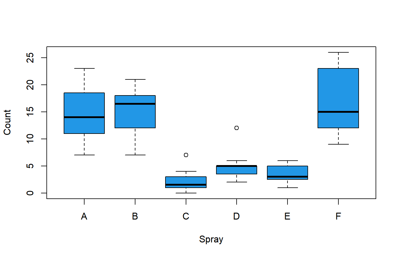
You can compute the sample variance of each group with tapply:
tapply(InsectSprays$count, InsectSprays$spray, var) A B C D E F
22.272727 18.242424 3.901515 6.265152 3.000000 38.606061The largest variance (spray F) is more than ten times the smallest one (spray E). Let’s see whether the tests confirm that the difference is significant.
Bartlett test with bartlett.test
The bartlett.test function is part of base R (stats package), so you don’t need to install anything. It accepts a formula or a list of numeric vectors, one per group:
bartlett.test(formula, data, subset, na.action, ...)

# Data and groups as vectors
bartlett.test(x, g, ...)

# A list with one numeric vector per group
bartlett.test(x, ...)
With the formula interface the response goes on the left and the grouping variable on the right:
bartlett.test(count ~ spray, data = InsectSprays) Bartlett test of homogeneity of variances
data: count by spray
Bartlett's K-squared = 25.96, df = 5, p-value = 9.085e-05If your data is stored in separate vectors, put them in a list. Using split you obtain the same list from a data frame, and the result is identical:
bartlett.test(split(InsectSprays$count, InsectSprays$spray))

# Equivalent to:
# bartlett.test(list(a, b, c, ...))
Bartlett test of homogeneity of variances
data: split(InsectSprays$count, InsectSprays$spray)
Bartlett's K-squared = 25.96, df = 5, p-value = 9.085e-05The output contains:
- Bartlett’s K-squared: the test statistic. The more different the group variances are, the larger it is.
- df: the degrees of freedom, the number of groups minus one (\(k - 1 = 5\)).
- p-value: computed from a chi-square distribution with \(k - 1\) degrees of freedom.
The p-value (0.00009) is far below 0.05, so you can reject the hypothesis of equal variances.
Bartlett is very sensitive to non-normality
The Bartlett test is the most powerful option when the data in each group is normal. The problem is that it can’t tell the difference between “different variances” and “non-normal data”: with skewed distributions or heavy tails it rejects the null hypothesis much more often than it should, even when all the variances are equal.
To see it, simulate three groups from the same exponential distribution. They have the same population variance (equal to 1), but the exponential distribution is strongly right-skewed:
set.seed(8)
df <- data.frame(group = gl(3, 30, labels = c("A", "B", "C")),
                 y = rexp(90, rate = 1))

hist(df$y, breaks = 20, col = 4, main = "", xlab = "y")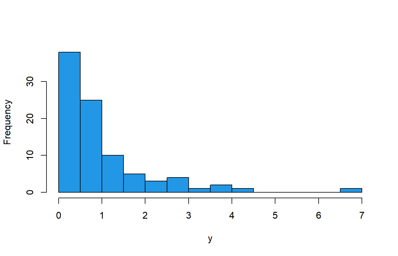
Now compare the results of both tests:
library(car)

bartlett.test(y ~ group, data = df)
leveneTest(y ~ group, data = df)
Bartlett test of homogeneity of variances
data: y by group
Bartlett's K-squared = 11.582, df = 2, p-value = 0.003055
Levene's Test for Homogeneity of Variance (center = median)
Df F value Pr(>F)
group 2 0.6885 0.505
87Bartlett rejects the equality of variances (p = 0.003) while Levene doesn’t (p = 0.505), and we know that the variances are actually equal. This is not bad luck in a single sample. If you repeat the simulation 1000 times you can count how often each test gives a p-value lower than 0.05:
# Proportion of p-values < 0.05 when all the variances are equal
set.seed(1)
res <- replicate(1000, {
  g <- gl(3, 30)
  y <- rexp(90)
  c(bartlett = bartlett.test(y ~ g)$p.value < 0.05,
    levene = leveneTest(y ~ g)[1, "Pr(>F)"] < 0.05)
})
rowMeans(res)
bartlett levene
0.382 0.044With a significance level of 0.05 a well-behaved test should reject about 5% of the times. Levene stays close to that (4.4%), while Bartlett rejects 38% of the times.
Use the Bartlett test only if you have checked that the data of each group is approximately normal (for instance with a Q-Q plot or the Shapiro-Wilk test). If you are not sure, use the Levene test.
Levene test with leveneTest
The leveneTest function belongs to the car package, so you will need to install it once with install.packages("car"). Its main arguments are:
library(car)

leveneTest(y, group, center = median, ...)

# With a formula
leveneTest(formula, data, center = median, ...)
Being:
y: numeric response variable (or a formula such asy ~ group).group: the factor that defines the groups.center: the function used to compute the center of each group,median(default) ormean.
The idea behind the test is simple: for each observation it computes the absolute deviation from the center of its group, \(z_{ij} = |y_{ij} - \tilde{y}_i|\), and then performs a one-way ANOVA on these deviations. If a group has more spread, its deviations will be larger on average.
library(car)

leveneTest(count ~ spray, data = InsectSprays)

# Equivalent to:
# leveneTest(InsectSprays$count, InsectSprays$spray)
Levene's Test for Homogeneity of Variance (center = median)
Df F value Pr(>F)
group 5 3.8214 0.004223 **
66
---
Signif. codes: 0 '***' 0.001 '**' 0.01 '*' 0.05 '.' 0.1 ' ' 1How to interpret the output
The output is a small ANOVA table:
- center = median: the heading tells you which center was used.
- Df: the first row (
group) contains the degrees of freedom of the groups (\(k - 1 = 5\)) and the second row the residual degrees of freedom (\(n - k = 72 - 6 = 66\)). - F value: the F statistic of the ANOVA on the absolute deviations (3.8214).
- Pr(>F): the p-value, obtained from an F distribution with 5 and 66 degrees of freedom.
The p-value is 0.0042 < 0.05, so the test rejects the null hypothesis of equal variances, the same conclusion as Bartlett.
You can check that it is just an ANOVA on the deviations from the median of each group with aov:
ins <- InsectSprays
ins$dev <- abs(ins$count - ave(ins$count, ins$spray, FUN = median))

summary(aov(dev ~ spray, data = ins))
Df Sum Sq Mean Sq F value Pr(>F)
spray 5 128.8 25.76 3.821 0.00422 **
Residuals 66 444.8 6.74
---
Signif. codes: 0 '***' 0.001 '**' 0.01 '*' 0.05 '.' 0.1 ' ' 1The F value and the p-value are the same. If you need the p-value inside your code, the result is a data frame, so you can extract it by position:
lt <- leveneTest(count ~ spray, data = InsectSprays)
lt[1, "Pr(>F)"]
[1] 0.004222791center = median vs center = mean
The original test proposed by Levene uses the mean of each group as the center. Brown and Forsythe proposed using the median instead, which makes the test more robust when the data is skewed. This is why leveneTest uses center = median by default, and many software packages call this version the Brown-Forsythe test.
To get the original Levene test set center = mean:
leveneTest(count ~ spray, data = InsectSprays, center = mean)Levene's Test for Homogeneity of Variance (center = mean)
Df F value Pr(>F)
group 5 6.4554 6.104e-05 ***
66
---
Signif. codes: 0 '***' 0.001 '**' 0.01 '*' 0.05 '.' 0.1 ' ' 1Here both versions reject the null hypothesis, but they can disagree with small or skewed samples. Keep the default (median) unless you have a reason to use the mean, and if you compare your results with other software (SPSS, for example, reports the version based on the mean) check which center was used.
Common mistake: a numeric grouping variable
In the ToothGrowth data set the dose (dose) is stored as a number (0.5, 1 and 2). If you use it as a group with the formula interface, leveneTest stops with an error:
leveneTest(len ~ dose, data = ToothGrowth)Error in leveneTest.formula(len ~ dose, data = ToothGrowth) :
Levene's test is not appropriate with quantitative explanatory variables.With the vector interface the test runs, but you get a warning telling you that the variable was converted to a factor:
leveneTest(ToothGrowth$len, ToothGrowth$dose)Levene's Test for Homogeneity of Variance (center = median)
Df F value Pr(>F)
group 2 0.6457 0.5281
57
Warning message:
In leveneTest.default(ToothGrowth$len, ToothGrowth$dose) :
ToothGrowth$dose coerced to factor.The result is correct in this case, but the clean solution is to convert the variable to a factor yourself before running the test, so you are sure that each value is treated as a group:
tg <- ToothGrowth
tg$dose <- factor(tg$dose)
Fligner-Killeen test with fligner.test
The Fligner-Killeen test is a non-parametric alternative available in base R. It works with the ranks of the absolute deviations from the median, so it is robust to non-normality and to outliers. Its syntax is the same as bartlett.test:
fligner.test(count ~ spray, data = InsectSprays)

# Equivalent to:
# fligner.test(split(InsectSprays$count, InsectSprays$spray))
Fligner-Killeen test of homogeneity of variances
data: count by spray
Fligner-Killeen:med chi-squared = 14.483, df = 5, p-value = 0.01282The p-value (0.0128) also leads to rejecting the equality of variances. As with Bartlett, the statistic is compared with a chi-square distribution with \(k - 1\) degrees of freedom. In the simulated skewed data of the previous section it doesn’t detect any difference either:
fligner.test(y ~ group, data = df) Fligner-Killeen test of homogeneity of variances
data: y by group
Fligner-Killeen:med chi-squared = 0.28484, df = 2, p-value = 0.8673Which test should you use?
The following table summarizes the three tests:
| Test | Function | Package | Assumes normality | When to use it |
|---|---|---|---|---|
| Bartlett | bartlett.test |
stats | Yes | Data clearly normal in each group (most powerful) |
| Levene / Brown-Forsythe | leveneTest |
car | No | Default choice, general use |
| Fligner-Killeen | fligner.test |
stats | No | Strong skewness or outliers, base R only |
| F test | var.test |
stats | Yes | Exactly two groups, also one-sided |
As a rule of thumb, use Levene (with the median) by default. Use Bartlett only when you are confident that the data is normal, and Fligner-Killeen when there are outliers or you don’t want to depend on extra packages.
With very large samples these tests detect tiny, irrelevant differences between variances, and with very small samples they have little power. Always look at the box plot and at the group variances as well: a ratio between the largest and smallest variance below 3 or 4 is usually not a problem for an ANOVA with groups of similar size.
Homogeneity of variances with several factors
In a two-way design, such as the two-way ANOVA, the variances to compare are those of each combination of factor levels. leveneTest accepts a formula with several factors and builds the groups from all the combinations (remember to convert dose to factor first):
tg <- ToothGrowth
tg$dose <- factor(tg$dose)

leveneTest(len ~ supp * dose, data = tg)
Levene's Test for Homogeneity of Variance (center = median)
Df F value Pr(>F)
group 5 1.7086 0.1484
54There are \(2 \times 3 = 6\) groups, so the test has 5 and 54 degrees of freedom. The p-value (0.1484) gives no evidence against equal variances.
bartlett.test and fligner.test only accept one grouping variable. If you write len ~ supp * dose you will get the error 'formula' should be of the form response ~ group. The solution is to create the combined groups with interaction:
bartlett.test(len ~ interaction(supp, dose), data = tg) Bartlett test of homogeneity of variances
data: len by interaction(supp, dose)
Bartlett's K-squared = 6.9273, df = 5, p-value = 0.2261What to do if the variances are not equal
Rejecting the homogeneity of variances doesn’t mean that you can’t compare the groups, only that you should use a method that doesn’t assume equal variances:
- Two groups: use the Welch t-test. It is the default of
t.test(var.equal = FALSE), so you only need to avoid settingvar.equal = TRUE. See the t-test tutorial for more details. - Three or more groups: use the Welch ANOVA with
oneway.test, as explained in the ANOVA tutorial. - Skewed data or outliers: a transformation of the response (such as the logarithm or the square root) often stabilizes the variances. The Kruskal-Wallis test is another option, but keep in mind that it is also affected when the shapes of the groups are very different.
For the InsectSprays data, where all the tests rejected the equality of variances, the Welch ANOVA is:
oneway.test(count ~ spray, data = InsectSprays) One-way analysis of means (not assuming equal variances)
data: count and spray
F = 36.065, num df = 5.000, denom df = 30.043, p-value = 7.999e-12The p-value is almost zero, so there is strong evidence that the mean number of insects is not the same for all the sprays, and this conclusion doesn’t rely on the assumption of equal variances.