Kruskal Wallis rank sum test (H test) in R

The kruskal.test function is used to perform the Kruskal-Wallis test in R, also known as H test or one-way ANOVA on ranks. This non-parametric test assesses whether there are statistically significant differences among two or more independent groups concerning their medians using ranked data. It is the generalization of the Wilcoxon test (also known as Mann-Whitney U test) for \(k\) independent samples.
The Kruskal-Wallis test is recommended when the data doesn’t meet the requirements to perform an ANOVA test.
Assumptions of the Kruskal-Wallis H Test
The Kruskal-Wallis test makes the following assumptions:
- Independence: observations within and between groups are independent.
- Ordinal or continuous data: the variable under study should be measured on an ordinal or continuous scale.
- Homogeneity of variance: the variance of the dependent variable should be approximately equal across groups.
- Random sampling: data should be obtained from a random sample from the population.
- Normality is not needed.
Check the homogeneity of variances with the Bartlett test (bartlett.test()) if the samples come from normal distributions or with the Levene test (leveneTest() from car package) if not.
Hypothesis
The Kruskal-Wallis test assesses whether there are differences in the distributions among groups based on location parameters. In essence, the null hypothesis assumes equal medians among groups, while the alternative hypothesis suggests inequality among medians. This is:
- \(H_0\): the medians among all groups are equal.
- \(H_1\): at least one group’s median is different from the others.
Syntax of kruskal.test
The syntax of the kruskal.test function is the following:
kruskal.test(x, g, ...)

# With a formula:
kruskal.test(formula, data, subset, na.action, ...)
Being:
x: numeric vector or list list of numeric vectors where each element is the data for a different group.g: character vector or factor containing the groups for the corresponding elements ofx. Ignored ifxis a list.formula: a formula object. The response variable is on the left-hand side, and the grouping variable is on the right-hand side.data: an optional data frame containing the variables used in the formula. If not provided, the variables should be present in the environment.subset: an optional vector specifying a subset of observations.na.action: function to deal with missing value....: further arguments to be passed.
Practical example
For this example we are going to utilize the chickwts data set, which provides 71 observations of chicken weights by feed type (6 groups).
The first step before performing a Kruskal-Wallis test is to make a previous exploratory data analysis:
# Sample data
df <- chickwts

# Box plot
boxplot(df$weight ~ df$feed, col = 4, xlab = "Group", ylab = "Value")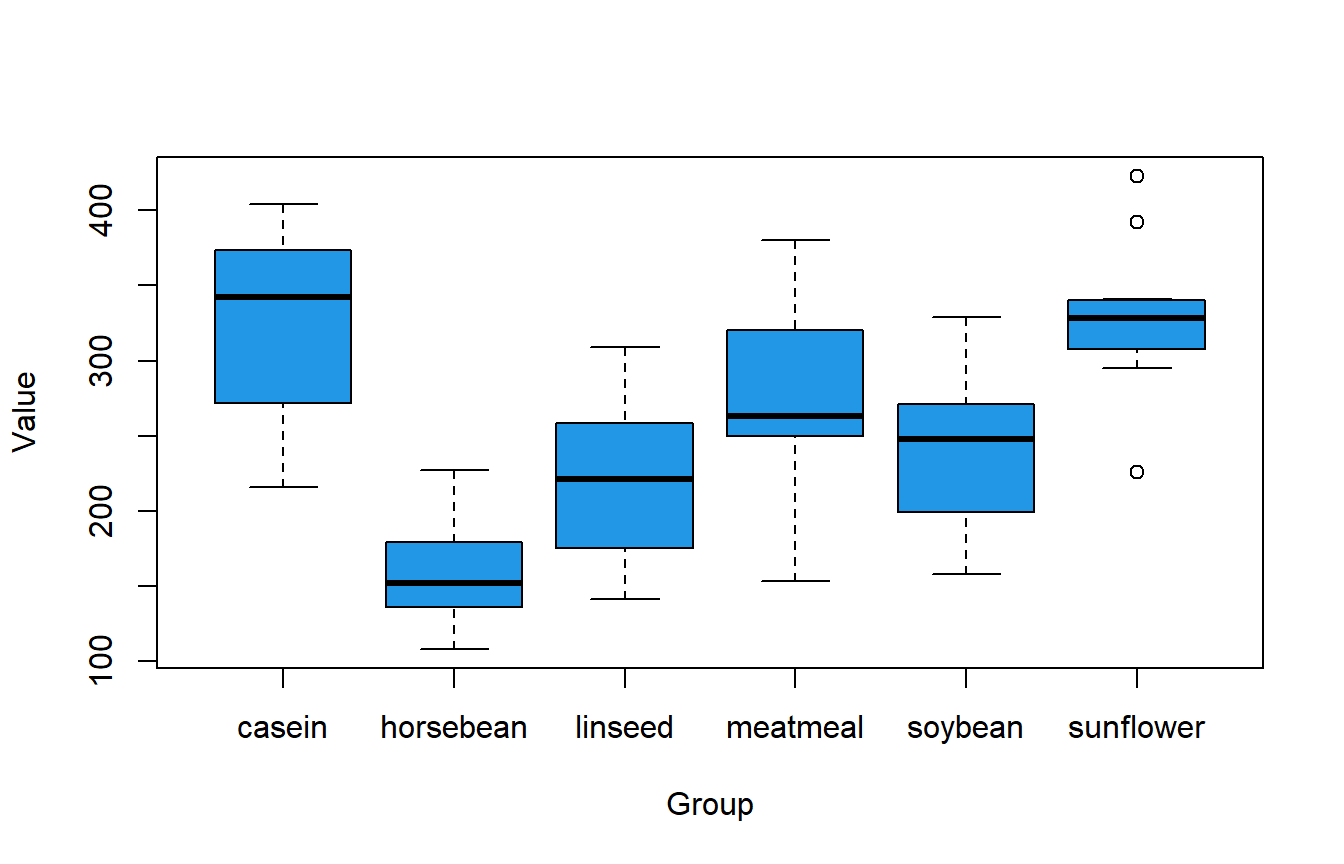
The previous box plot illustrates potential differences among groups. Moreover, employing the tapply function enables the creation of sample summary statistics, such as the minimum and maximum values, the mean, and the quartiles by group.
# Sample data
df <- chickwts

tapply(df$weight, df$feed, summary)
$casein
Min. 1st Qu. Median Mean 3rd Qu. Max.
216.0 277.2 342.0 323.6 370.8 404.0
$horsebean
Min. 1st Qu. Median Mean 3rd Qu. Max.
108.0 137.0 151.5 160.2 176.2 227.0
$linseed
Min. 1st Qu. Median Mean 3rd Qu. Max.
141.0 178.0 221.0 218.8 257.8 309.0
$meatmeal
Min. 1st Qu. Median Mean 3rd Qu. Max.
153.0 249.5 263.0 276.9 320.0 380.0
$soybean
Min. 1st Qu. Median Mean 3rd Qu. Max.
158.0 206.8 248.0 246.4 270.0 329.0
$sunflower
Min. 1st Qu. Median Mean 3rd Qu. Max.
226.0 312.8 328.0 328.9 340.2 423.0 Now you will have to test for equal variances among groups. For this purpose, you can use the Bartlett (normality is required) or Levene test, which is more robust:
# Sample data
df <- chickwts

library(car)
leveneTest(df$weight ~ df$feed)
Levene's Test for Homogeneity of Variance (center = median)
Df F value Pr(>F)
group 5 0.7493 0.5896
65 The test return a p-value greater than the usual significance levels, so there is no statistical evidence to reject the null hypothesis of homogeneity of variances.
Once you know the data meets the assumptions you can perform the Kruskal-Wallis test with the kruskal.test function as follows:
# Sample data
df <- chickwts

# Is the median of 'weight' equal among all groups of 'feed'?
kruskal.test(df$weight ~ df$feed)

# Equivalent to:
# kruskal.test(weight ~ feed, data = df)
# kruskal.test(x = df$weight, g = df$feed)
# kruskal.test(x = split(df$weight, df$feed, drop = TRUE)) # List
Kruskal-Wallis rank sum test
data: df$weight by df$feed
Kruskal-Wallis chi-squared = 37.343, df = 5, p-value = 5.113e-07The p-value is close to zero, implying strong evidence against the null hypothesis of equal median among groups.
The Kruskal-Wallis test doesn’t tell you which specific group differs; it only determines if there is a significant difference among groups. Further post-hoc tests or pairwise comparisons might be needed to identify specific group differences after rejecting the null hypothesis.
Post-hoc comparisons
The output of the Kruskal-Wallis test indicates evidence that the group medians are not equal. However, this test does not specify which groups differ. To identify the differing groups, you can use the pairwise.wilcox.test function, which conducts Wilcoxon tests for each pair of groups.
pairwise.wilcox.test(x = df$weight, g = df$feed) Pairwise comparisons using Wilcoxon rank sum exact test
data: df$weight and df$feed
casein horsebean linseed meatmeal soybean
horsebean 0.00030 - - - -
linseed 0.01221 0.05001 - - -
meatmeal 0.36337 0.00306 0.21806 - -
soybean 0.04736 0.00834 0.70996 0.70996 -
sunflower 1.00000 9.3e-05 0.00064 0.34409 0.01402
P value adjustment method: holm The function will return a matrix of p-values. If the corresponding p-value is lower than the usual significance levels, then there is strong evidence against the equality of medians for that pair of groups. For instance, the first p-value (0.00030) indicates that the groups named horsebean and casein do not have the same median.