Barplot in R

When a variable takes a few values, it is common to summarize the information with a frequency table that can be represented with a barchart or barplot in R. In this article we are going to explain the basics of creating bar plots in R.
R’s barplot() function
For creating a barplot in R you can use the base R barplot function. In this example, we are going to create a bar plot from a data frame. Specifically, the example dataset is the well-known mtcars. First, load the data and create a table for the cyl column with the table function.
# Load data
data(mtcars)
attach(mtcars)

# Frequency table
my_table <- table(cyl)
my_table
cyl
4 6 8
11 7 14Recall that to create a barplot in R you can use the barplot function setting as a parameter your previously created table to display absolute frequency of the data. However, if you prefer a bar plot with percentages in the vertical axis (the relative frequency), you can use the prop.table function and multiply the result by 100 as follows.
# One row, two columns
par(mfrow = c(1, 2))

# Absolute frequency barplot
barplot(my_table, main = "Absolute frequency",
        col = rainbow(3))

# Relative frequency barplot
barplot(prop.table(my_table) * 100, main = "Relative frequency (%)",
        col = rainbow(3))

par(mfrow = c(1, 1))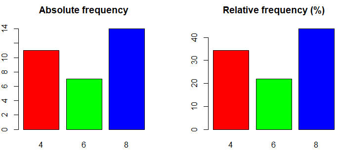
Note that you can also create a barplot with factor data with the plot function.
plot(factor(mtcars$cyl), col = rainbow(3))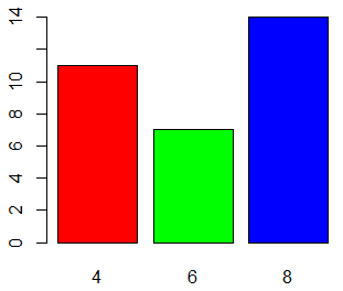
In addition, you can show numbers on bars with the text function as follows:
barp <- barplot(my_table, col = rainbow(3), ylim = c(0, 15))
text(barp, my_table + 0.5, labels = my_table)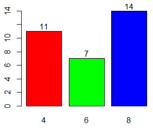
Assigning a bar plot inside a variable will store the axis values corresponding to the center of each bar.
You can also add a grid behind the bars with the grid function.
barp <- barplot(my_table, col = rainbow(3), ylim = c(0, 15))
grid(nx = NA, ny = NULL, lwd = 1, lty = 1, col = "gray")
barplot(my_table, col = rainbow(3), ylim = c(0, 15), add = TRUE)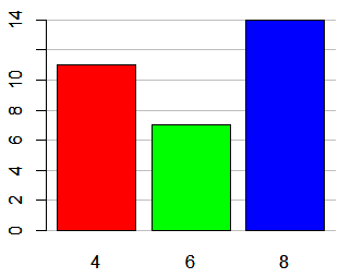
Barplot graphical parameters: title, axis labels and colors
Like other plots, you can specify a wide variety of graphical parameters, like axis labels, a title or customize the axes. In the previous code block we customized the barplot colors with the col parameter. You can set the colors you prefer with a vector or use the rainbow function with the number of bars as parameter as we did or use other color palette functions. You can also change the border color of the bars with the border argument.
barplot(my_table,                               # Data
        main = "Customized bar plot",           # Title
        xlab = "Number of cylinders",           # X-axis label
        ylab = "Frequency",                     # Y-axis label
        border = "black",                       # Bar border colors
        col = c("darkgrey", "darkblue", "red")) # Bar colors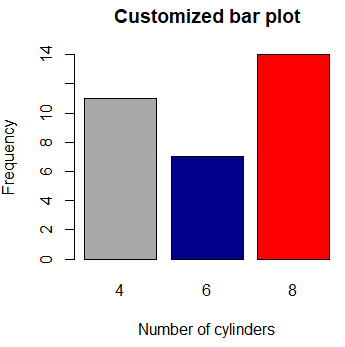
Change group labels
The label of each group can be changed with the names.arg argument. In our example, the groups are labelled with numbers, but we can change them typing something like:
barplot(my_table, names.arg = c("four", "six", "eight")) 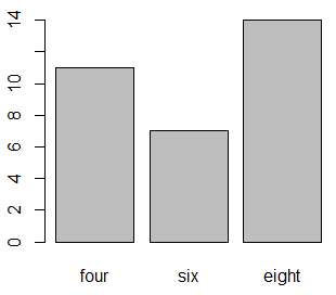
Barplot width and space of bars
You can also modify the space between bars or the width of the bars with the width and space arguments. For the space between groups, consult the corresponding section of this tutorial.
par(mfrow = c(1, 2))

# Bar width (by default: width = 1)
barplot(my_table, main = "Change bar width",
        col = rainbow(3), width = c(0.4, 0.2, 1))

# Bar space
barplot(my_table, main = "Change space between bars",
        col = rainbow(3), space = c(1, 1.1, 0.1))

par(mfrow = c(1, 1))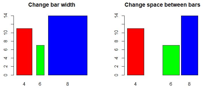
The space vector represents the space of the bar respect to the previous, so the first element won’t be taken into account.
Barplot from data frame or list
In addition, you can create a barplot directly with the variables of a dataframe or even a matrix, but note that the variable should be the count of some event or characteristic. In the following example we are counting the number of vehicles by color and plotting them with a bar chart. We will use each car color for coloring the corresponding bars.
df <- data.frame(carColor = c("red", "green", "white", "blue"),
                 count = c(3, 5, 9, 1))
# df <- as.list(df) # Equivalent

barplot(height = df$count, names = df$carColor,
        col = c("red", "green", "white", "blue"))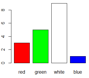
Barplot for continuous variable
In case you are working with a continuous variable you will need to use the cut function to categorize the data. If not, in case of no ties, you will have as many bars as the length of your vector and the bar heights will equal to 1. In the following example we will divide our data from 0 to 45 by steps of 5 with the breaks argument.
x <- c(2.1, 8.6, 3.9, 4.4, 4.0, 3.7, 7.6, 3.1, 5.0, 5.5, 20.2, 1.7,
       5.2, 33.7, 9.1, 1.6, 3.1, 5.6, 16.5, 15.8, 5.8, 6.8, 3.3, 40.6)

barplot(table(cut(x, breaks = seq(0, 45, by = 5))))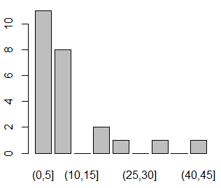
Horizontal barplot
By default, barplots in R are plotted vertically. However, it is common to represent horizontal bar plots. You can rotate 90º the plot and create a horizontal bar chart setting the horiz argument to TRUE.
barplot(my_table, main = "Barchart",
        ylab = "Number of cylinders", xlab = "Frequency",
        horiz = TRUE) # Horizontal barplot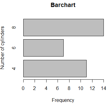
R barplot legend
A legend can be added to a barplot in R with the legend.text argument, where you can specify the names you want to add to the legend. Note that in RStudio the resulting plot can be slightly different, as the background of the legend will be white instead of transparent.
barplot(my_table, xlab = "Number of cylinders",
        col = rainbow(3),
        legend.text = rownames(my_table)) # Legend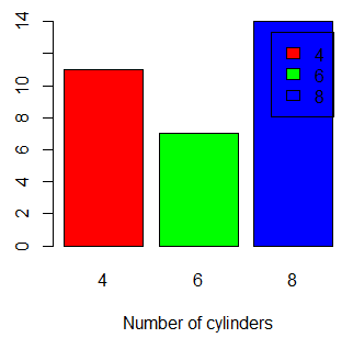
Note that, by using the legend.text argument, the legend can overlap the barplot.
The easiest method to solve this issue in this example is to move the legend. This can be achieved with the args.legend argument, where you can set graphical parameters within a list. You can set the position to top, bottom, topleft, topright, bottomleft and bottomright.
barplot(my_table, xlab = "Number of cylinders",
        col = rainbow(3),
        legend.text = rownames(my_table),
        args.legend = list(x = "top"))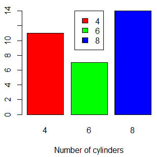
Equivalently, you can achieve the previous plot with the legend with the legend function as follows with the legend and fill arguments.
barplot(my_table, xlab = "Number of cylinders",
        col = rainbow(3))
legend("top", legend = rownames(my_table), fill = rainbow(3))
Nevertheless, this approach only works fine if the legend doesn’t overlap the bars in those positions. A better approach is to move the legend to the right, out of the barplot. You can do this setting the inset argument passed as a element of a list within the args.legend argument as follows.
par(mar = c(5, 5, 4, 10))
barplot(my_table, xlab = "Number of cylinders",
        col = rainbow(3),
        legend.text = rownames(my_table), # Legend values
        args.legend = list(x = "topright", inset = c(-0.20, 0))) # Legend arguments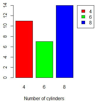
You could also change the axis limits with the xlim or ylim arguments for vertical and horizontal bar charts, respectively, but note that in this case the value to specify will depend on the number and the width of bars. Recall that if you assign a barplot to a variable you can store the axis points that correspond to the center of each bar.
barplot(my_table, xlab = "Number of cylinders",
        col = rainbow(3),
        legend.text = rownames(my_table), xlim = c(0, 4.25))
Other alternative to move the legend is to move it under the bar chart with the layout, par and plot.new functions. This approach is more advanced than the others and you may need to clear the graphical parameters before the execution of the code to obtain the correct plot, as graphical parameters will be changed.
# dev.off()
# opar <- par(no.readonly = TRUE)
plot.new()
layout(rbind(1, 2), heights = c(10, 3))
barplot(my_table, xlab = "Number of cylinders",
        col = rainbow(3))

par(mar = c(0, 0, 0, 0))
plot.new()
legend("top", rownames(my_table), lty = 1,
       col = c("red", "green", "blue"), lwd = c(1, 2))
# dev.off()
# on.exit(par(opar))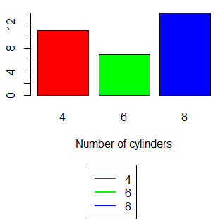
Grouped barplot in R
A grouped barplot, also known as side by side bar plot or clustered bar chart is a barplot in R with two or more variables. The chart will display the bars for each of the multiple variables.
# Variable am to factor
am <- factor(am)

# Change factor levels
levels(am) <- c("Automatic", "Manual")

# Table cylinder - transmission type
other_table <- table(cyl, am)
# other_table <- xtabs(~cyl + am , data = mtcars) # Equivalent

barplot(other_table,
        main = "Grouped barchart",
        xlab = "Transmission type", ylab = "Frequency",
        col = c("darkgrey", "darkblue", "red"),
        legend.text = rownames(other_table),
        beside = TRUE) # Grouped bars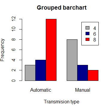
Note that if we had specified table(am, cyl) instead of table(cyl, am) the X-axis would represent the number of cylinders instead of the transmission type.
Space between groups
As we reviewed before, you can change the space between bars. In the case of several groups you can set a two-element vector where the first element is the space between bars of each group (0.4) and the second the space between groups (2.5).
barplot(other_table,
        main = "Grouped barchart space",
        xlab = "Transmission type", ylab = "Frequency",
        col = c("darkgrey", "darkblue", "red"),
        legend.text = rownames(other_table),
        beside = TRUE,
space = c(0.4, 2.5)) # Space 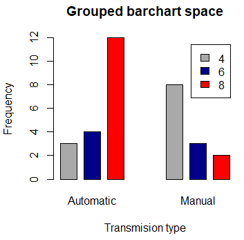
Numeric values in groups
Barplots also can be used to summarize a variable in groups given by one or several factors. Consider, for instance, that you want to display the number of cylinders and transmission type based on the mean of the horse power of the cars. You could use the tapply function to create the corresponding table:
summary_data <- tapply(mtcars$hp, list(cylinders = mtcars$cyl,
                                       transmission = mtcars$am),
                       FUN = mean, na.rm = TRUE)
summary_data
transmission
cylinders Automatic Manual
4 84.66667 81.8750
6 115.25000 131.6667
8 194.16667 299.5000Now, you can create the corresponding barplot in R:
par(mar = c(5, 5, 4, 10))

barplot(summary_data, xlab = "Transmission type",
        main = "Horsepower mean",
        col = rainbow(3),
        beside = TRUE,
        legend.text = rownames(summary_data),
        args.legend = list(title = "Cylinders", x = "topright",
                           inset = c(-0.20, 0)))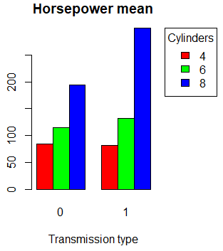
Barplot with error bars in R
By default, you can’t create a barplot with error bars. However, the following function will allow you to create a fully customizable barplot with standard error bars.
# Arguments:
# x: an unique factor object
# y: a numeric vector object
# ...: additional arguments to be passed to barplot function

barplot.error <- function(x, y, ...){
    mod <- lm(y ~ x)
    reps <- sqrt(length(y)/length(levels(x)))
    sem <- sigma(mod)/reps
    means <- tapply(y, x, mean)
    upper <- max(means) + sem
    lev <- levels(x)
    barpl <- barplot(means, ...)
    invisible(sapply(1:length(barpl), function(i) arrows(barpl[i], means[i] + sem,
              barpl[i], means[i] - sem, angle = 90, code = 3, length = 0.08)))
}

# Calling the function
barplot.error(factor(mtcars$cyl), mtcars$hp, col = rainbow(3), ylim = c(0, 250))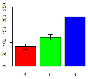
Even you can add error bars to a barplot, it should be noticed that a boxplot by group could be a better approach to summarize the data in this scenario.
Stacked barplot in R
A stacked bar chart is like a grouped bar graph, but the frequency of the variables are stacked. This type of barplot will be created by default when passing as argument a table with two or more variables, as the argument beside defaults to FALSE.
barplot(other_table,
        main = "Stacked barchart",
        xlab = "Transmission type", ylab = "Frequency",
        col = c("darkgrey", "darkblue", "red"),
        legend.text = rownames(other_table),
        beside = FALSE) # Stacked bars (default)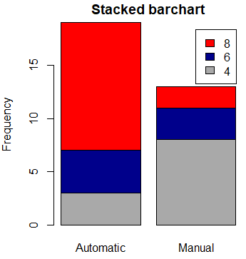
Related to stacked bar plots, there exists similar implementations, like the spine plot and mosaic plot. This type of plots can be created with the spineplot and mosaicplot functions of the graphics package.
The mosaic plot allows you to visualize data of two or more quantitative variables, where the area of each rectangle represents the proportion of that variable on each group.
# install.packages("graphics")
library(graphics)

mosaicplot(other_table, main = "Mosaic plot")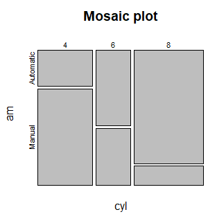
The spineplot is a special case of a mosaic plot, and its a generalization of the stacked barplot. In this case, unlike stacked barplots, each bar sums up to one.
spineplot(other_table)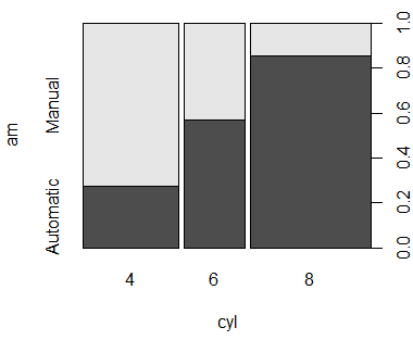
Note that, by default, axes are interchanged with respect to the stacked bar plot you created in the previous section. You can create the equivalent plot transposing the frequency table with the t function.
spineplot(t(other_table))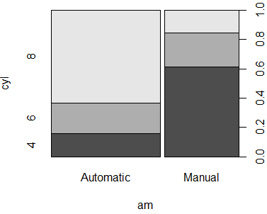
Barplot in R: ggplot2
The ggplot2 library is a well know graphics library in R. You can create a barplot with this library converting the data to data frame and with the ggplot and geom_bar functions. In the aes argument you have to pass the variable names of your dataframe. In x the categorical variable and in y the numerical.
# install.packages("ggplot2")
library(ggplot2)

df <- as.data.frame(my_table)

ggplot(data = df, aes(x = cyl, y = Freq)) +
       geom_bar(stat = "identity")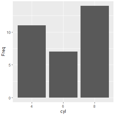
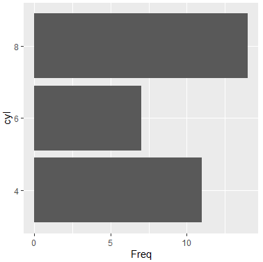
Horizontal barplot ggplot2
If you want to rotate the previous barplot use the coord_flip function as follows.
ggplot(data = df, aes(x = cyl, y = Freq)) +
       geom_bar(stat = "identity") +
       coord_flip() # Horizontal bar plot