Chi-square distribution in R
The chi-square (\(\chi^2\)) distribution is the reference distribution of the chi-squared tests and of the confidence interval for a variance. In this tutorial you will learn how to use the dchisq, pchisq, qchisq and rchisq functions in R, how to get the p-value from a chi-square statistic (and avoid the most common mistake), how to find chi-square critical values and how to compute a confidence interval for the variance by hand.
The chi-square distribution
If \(Z_1, Z_2, \dots, Z_k\) are independent standard normal random variables, the sum of their squares
\[X = Z_1^2 + Z_2^2 + \dots + Z_k^2\]
follows a chi-square distribution with \(k\) degrees of freedom (df), denoted as \(X \sim \chi^2_k\). The degrees of freedom are the only parameter of the distribution. Then:
- It only takes non-negative values, as it is a sum of squares.
- It is right-skewed, and the skewness decreases as the degrees of freedom increase.
- The expected mean and variance are \(E(X) = k\) and \(Var(X) = 2k\).
- For a large number of degrees of freedom it approaches a normal distribution with mean \(k\) and variance \(2k\).
You will find this distribution behind the Pearson’s chi-squared test, the Kruskal-Wallis test statistic and the confidence interval for the variance of a normal population. In R, the functions related to the chi-square distribution are the following:
| Function | Description | Typical use |
|---|---|---|
| dchisq |
Chi-square density (Probability Density Function) |
Plot the curve |
| pchisq |
Chi-square distribution (Cumulative Distribution Function) |
p-values |
| qchisq | Quantile function of the chi-square distribution | Critical values and confidence intervals |
| rchisq | Chi-square random number generation | Simulation |
The dchisq function
The dchisq function returns the density of the chi-square distribution. The syntax is the following:
dchisq(x,           # Vector of values (quantiles)
       df,          # Degrees of freedom (non-negative, can be non-integer)
       ncp = 0,     # Non-centrality parameter
       log = FALSE) # If TRUE, densities are given as log
For instance, the density of a chi-square with 3 degrees of freedom at 0.5, 1, 2 and 5 is:
dchisq(c(0.5, 1, 2, 5), df = 3)[1] 0.21969564 0.24197072 0.20755375 0.07322491Recall that a density is not a probability. For example, dchisq(0, df = 1) returns Inf, because the curve with 1 degree of freedom goes to infinity at zero, while with 2 df the density at zero is 0.5 and with 3 or more df it is 0.
Plot the chi-square distribution in R
The shape of the distribution changes a lot with the degrees of freedom. The following code plots the density for 1, 2, 3, 5 and 10 degrees of freedom with a for loop:
# Grid of X-axis values
x <- seq(0, 20, length = 300)

dfs <- c(1, 2, 3, 5, 10)
cols <- c("red", "orange", "darkgreen", "blue", "purple")

# Empty plot
plot(x, dchisq(x, df = 1), type = "n", ylim = c(0, 0.5),
     xlab = "x", ylab = "Density")

# One line for each df
for (i in seq_along(dfs)) {
  lines(x, dchisq(x, df = dfs[i]), lwd = 2, col = cols[i])
}

legend("topright", legend = paste("df =", dfs), col = cols,
       lwd = 2, box.lty = 0)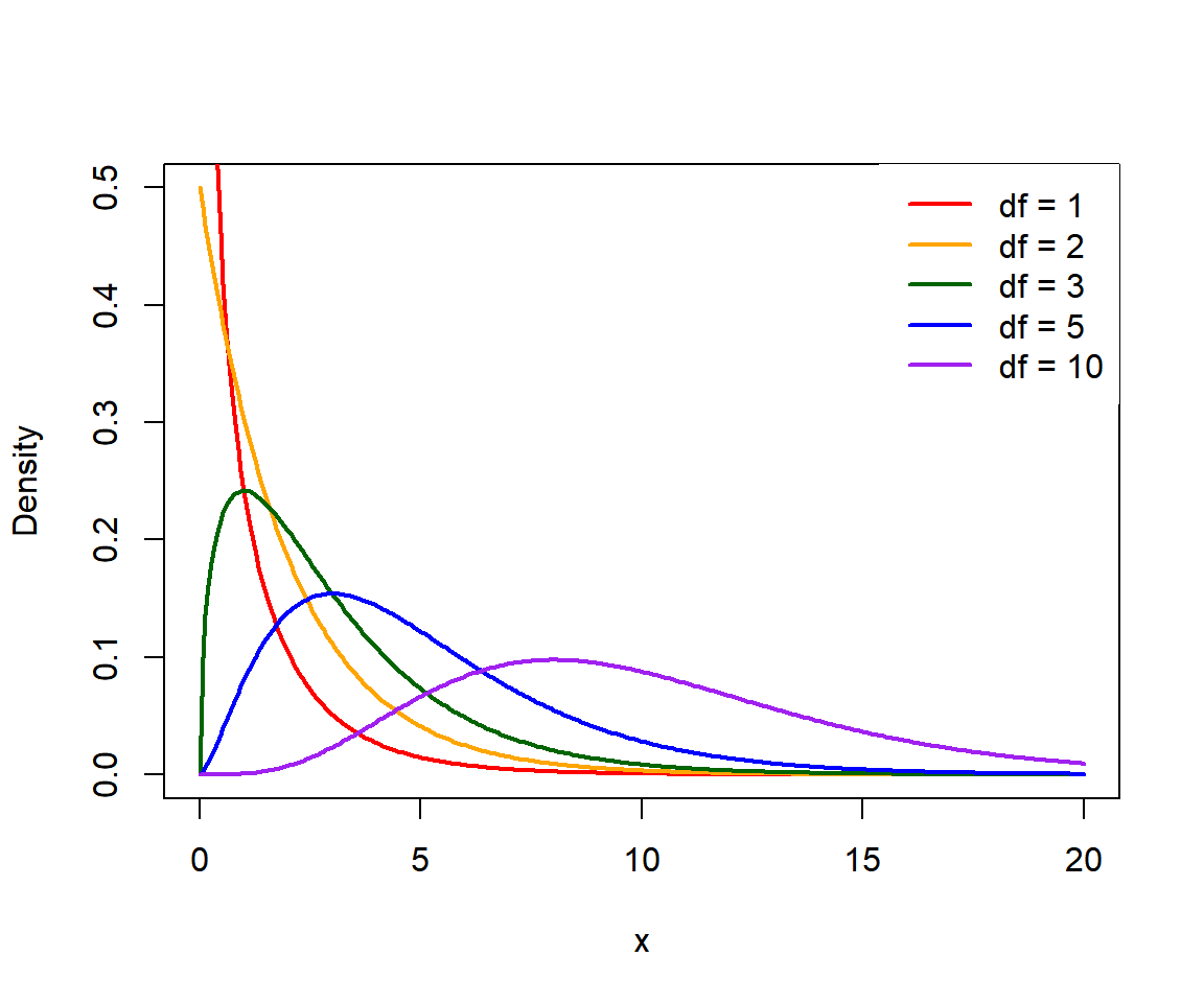
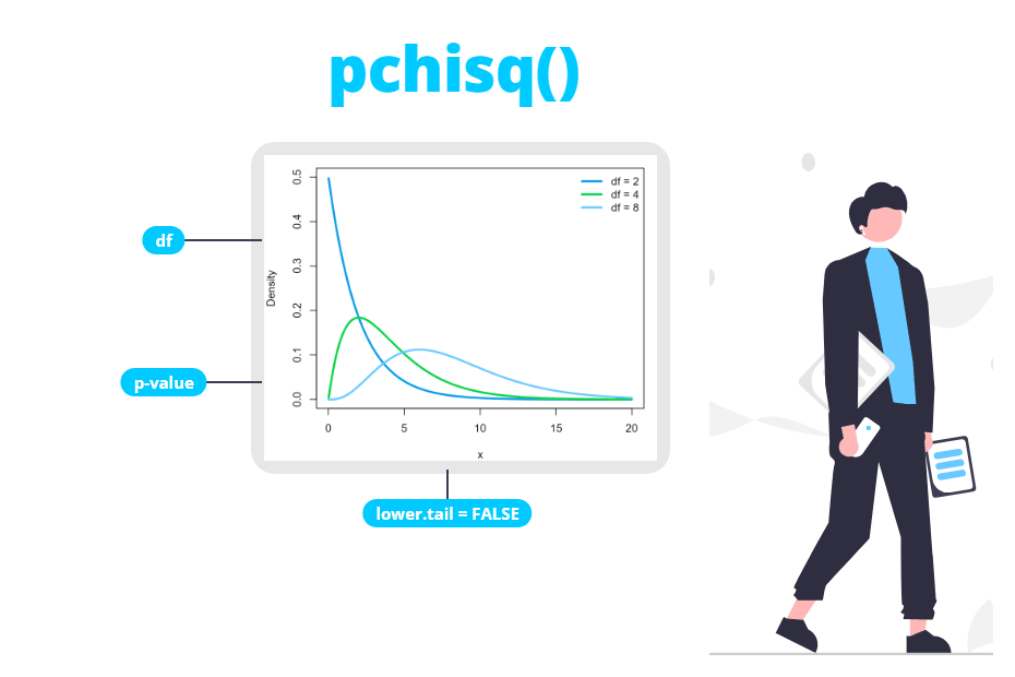
With 1 and 2 degrees of freedom the density is decreasing. From 3 df on the curve has a peak (the mode is \(k - 2\)) and, as \(k\) increases, it moves to the right and becomes more symmetric.
The pchisq function
The pchisq function gives the cumulative distribution function, \(P(X \leq q)\). With lower.tail = FALSE it returns the upper tail, \(P(X > q)\).
pchisq(q,                 # Vector of quantiles
       df,                # Degrees of freedom
       ncp = 0,           # Non-centrality parameter
       lower.tail = TRUE, # If TRUE, P(X <= q), or P(X > q) otherwise
       log.p = FALSE)     # If TRUE, probabilities are given as log
For example, the probability that a chi-square with 3 df is lower or equal than 3 and the probability that it is greater than 3:
pchisq(3, df = 3)                     # P(X <= 3)
pchisq(3, df = 3, lower.tail = FALSE) # P(X > 3)
[1] 0.6083748
[1] 0.3916252P-value from a chi-square statistic
In the chi-squared tests, large values of the statistic are evidence against the null hypothesis, so the p-value is always the upper tail probability, \(P(X > \chi^2_{obs})\).
Consider the example of the chi-squared test for independence between price and quality of 100 products:
data <- matrix(c(40, 20, 10, 30), nrow = 2)
rownames(data) <- c("High price", "Low price")
colnames(data) <- c("High quality", "Low quality")

chi <- chisq.test(data)
chi
Pearson's Chi-squared test with Yates' continuity correction
data: data
X-squared = 15.042, df = 1, p-value = 0.0001052You can access the statistic and the degrees of freedom with chi$statistic and chi$parameter and compute the p-value with pchisq:
# Upper tail: P(X > statistic)
pchisq(chi$statistic, df = chi$parameter, lower.tail = FALSE)
X-squared
0.0001051636The result is the same p-value returned by chisq.test. This is useful when you only have the statistic, for example from a paper or from another software, and you need the p-value.
The most common mistake is to forget lower.tail = FALSE. pchisq(15.042, df = 1) returns 0.9998949, which is one minus the p-value, and leads to the opposite conclusion. Unlike the t-test, you don’t multiply by 2: the chi-squared tests are one-tailed by construction.
The qchisq function
The qchisq function is the inverse of pchisq: it returns the value \(q\) that leaves a probability \(p\) to its left. Its main uses are critical values and confidence intervals.
qchisq(p,                 # Vector of probabilities
       df,                # Degrees of freedom
       ncp = 0,           # Non-centrality parameter
       lower.tail = TRUE, # If TRUE, probabilities are P(X <= x), or P(X > x) otherwise
       log.p = FALSE)     # If TRUE, probabilities are given as log
Chi-square critical values
As the rejection region of a chi-squared test is in the upper tail, the critical value at a significance level \(\alpha\) is the quantile \(1 - \alpha\):
qchisq(0.95, df = 1)                     # alpha = 0.05, df = 1
qchisq(0.05, df = 1, lower.tail = FALSE) # Equivalent
qchisq(0.95, df = 3)                     # alpha = 0.05, df = 3
[1] 3.841459
[1] 3.841459
[1] 7.814728Note that \(3.841 = 1.96^2\): with one degree of freedom the chi-square is the square of a standard normal, so qchisq(0.95, 1) is equal to qnorm(0.975)^2.
Let’s see how to use the critical value in a goodness-of-fit test. Suppose that 100 customers chose among four product colors and you want to test if all colors are equally popular:
obs <- c(25, 18, 22, 35)
chisq.test(obs)
Chi-squared test for given probabilities
data: obs
X-squared = 6.32, df = 3, p-value = 0.09704The statistic (6.32) is lower than the critical value with 3 df (7.815), so you don’t reject the null hypothesis at the 5% level. Both approaches always lead to the same decision: statistic greater than the critical value is the same as p-value lower than \(\alpha\).
The following code creates a table with the critical values for several degrees of freedom and significance levels:
dfs <- c(1:10, 15, 20, 30)
alpha <- c(0.10, 0.05, 0.01)

crit <- sapply(alpha, function(a) qchisq(1 - a, df = dfs))
dimnames(crit) <- list(df = dfs, alpha = alpha)
round(crit, 3)
alpha
df 0.1 0.05 0.01
1 2.706 3.841 6.635
2 4.605 5.991 9.210
3 6.251 7.815 11.345
4 7.779 9.488 13.277
5 9.236 11.070 15.086
6 10.645 12.592 16.812
7 12.017 14.067 18.475
8 13.362 15.507 20.090
9 14.684 16.919 21.666
10 15.987 18.307 23.209
15 22.307 24.996 30.578
20 28.412 31.410 37.566
30 40.256 43.773 50.892Confidence interval for the variance
If the data come from a normal population, \((n-1)s^2/\sigma^2\) follows a chi-square distribution with \(n - 1\) degrees of freedom. Hence, the confidence interval for the variance \(\sigma^2\) with confidence level \(1 - \alpha\) is
\[\left( \frac{(n-1)s^2}{\chi^2_{1-\alpha/2,\, n-1}}, \frac{(n-1)s^2}{\chi^2_{\alpha/2,\, n-1}} \right)\]
Note that the interval is not symmetric around \(s^2\), as the chi-square distribution isn’t. R doesn’t have a base function for this interval, but you can compute it with qchisq and var. For the mpg variable of mtcars:
x <- mtcars$mpg
n <- length(x)
s2 <- var(x) # 36.3241

alpha <- 0.05
lower <- (n - 1) * s2 / qchisq(1 - alpha / 2, df = n - 1)
upper <- (n - 1) * s2 / qchisq(alpha / 2, df = n - 1)

# Interval for the variance
c(lower, upper)

# Interval for the standard deviation
sqrt(c(lower, upper))
[1] 23.34653 64.20343
[1] 4.831825 8.012704So the true variance is between 23.35 and 64.20 with a 95% confidence, and the standard deviation (sample value 6.03) between 4.83 and 8.01. Notice how wide the interval is with 32 observations: variances are estimated with much less precision than means.
Unlike the confidence interval for the mean, this interval is very sensitive to non-normality, even with large samples. Check the normality of the data first, for instance with the Shapiro-Wilk test.
The rchisq function
The rchisq function generates random observations from a chi-square distribution. Use set.seed to make the results reproducible:
rchisq(n,       # Number of observations to be generated
       df,      # Degrees of freedom
       ncp = 0) # Non-centrality parameter
set.seed(1)
rchisq(5, df = 3)[1] 0.9433146 5.5437816 5.3543968 2.9152466 5.0531908A nice way to understand the definition of the distribution is to simulate it. The following code generates 100000 sums of three squared standard normal values and compares their mean and variance with those of rchisq with 3 degrees of freedom. Theory says that both should be close to \(k = 3\) and \(2k = 6\):
set.seed(1)

# Sum of 3 squared standard normals
z <- matrix(rnorm(100000 * 3), ncol = 3)
q <- rowSums(z^2)

# Chi-square with 3 df
y <- rchisq(100000, df = 3)

c(mean = mean(q), var = var(q))
c(mean = mean(y), var = var(y))
mean var
3.004272 6.028960
mean var
2.990382 5.948571Both simulations give a mean close to 3 and a variance close to 6. You can also check it visually with a histogram of the simulated sums and the theoretical density on top:
set.seed(1)
z <- matrix(rnorm(100000 * 3), ncol = 3)
q <- rowSums(z^2)

hist(q, breaks = 60, prob = TRUE, col = "lightgray", border = "white",
     main = "", xlab = "Sum of 3 squared N(0, 1)", xlim = c(0, 20))
curve(dchisq(x, df = 3), add = TRUE, lwd = 2, col = "red")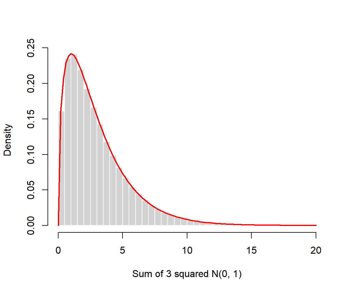
The red curve fits the histogram perfectly. Finally, all the functions accept the ncp argument for the non-central chi-square distribution, which is the distribution of the test statistic when the null hypothesis is false and is used in power calculations.