Fisher's exact test in R with fisher.test()
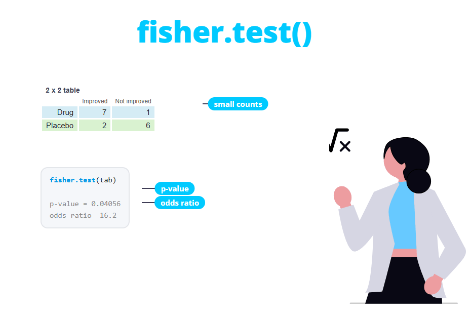
The fisher.test function performs Fisher’s exact test in R, which checks whether two categorical variables are independent using the exact probabilities of the contingency table instead of an approximation. It is the test to use when the sample is small and the chi-squared test is not reliable. In this tutorial you will learn when to use it, how to interpret its p-value, odds ratio and confidence interval, how to run one-sided tests and what to do with larger tables.
When to use Fisher’s exact test
The chi-squared test compares the observed counts of a contingency table with the counts you would expect if the variables were independent. Its p-value comes from an approximation to the chi-square distribution, and that approximation is poor when the expected counts are small.
Consider a small clinical trial with 16 patients: 8 received a drug and 8 a placebo, and you recorded whether they improved:
trt <- matrix(c(7, 2, 1, 6), nrow = 2,
              dimnames = list(Treatment = c("Drug", "Placebo"),
                              Outcome = c("Improved", "Not improved")))
trt
Outcome
Treatment Improved Not improved
Drug 7 1
Placebo 2 6If you run chisq.test on this table, R gives you a result but also a warning:
chi <- chisq.test(trt)
chi
Warning message:
In chisq.test(trt) : Chi-squared approximation may be incorrect
Pearson's Chi-squared test with Yates' continuity correction
data: trt
X-squared = 4.0635, df = 1, p-value = 0.04382The warning “Chi-squared approximation may be incorrect” appears when at least one expected count is lower than 5. You can check the expected counts with the expected element of the result:
chi$expected Outcome
Treatment Improved Not improved
Drug 4.5 3.5
Placebo 4.5 3.5All four expected counts are below 5. The usual rule says that the chi-squared approximation is acceptable if all the expected counts are at least 5 (a more relaxed version allows up to 20% of the cells below 5 and none below 1). When the rule fails, use Fisher’s exact test.
The rule is about the expected counts, not the observed ones. A table can have a cell with an observed count of 0 and still be fine for the chi-squared test if all its expected counts are 5 or greater.
Hypotheses
Fisher’s exact test has the same hypotheses as the chi-squared test of independence:
- \(H_0\): the two variables are independent (in a 2x2 table, the odds ratio is equal to 1).
- \(H_1\): the two variables are not independent (the odds ratio is different from 1).
The test considers the row and column totals as fixed and computes the exact probability of obtaining each possible table with those totals, using the hypergeometric distribution. The p-value is the sum of the probabilities of all the tables that are as unlikely as the observed one or more. This is why it is called “exact”: it doesn’t rely on any large-sample approximation.
Syntax of fisher.test
The main arguments of the function are the following:
fisher.test(x, y = NULL, alternative = "two.sided",
            conf.int = TRUE, conf.level = 0.95,
            simulate.p.value = FALSE, B = 2000, workspace = 200000, ...)
Being:
x: a contingency table or a matrix with the counts, or a factor.y: a factor with the second variable. Ignored ifxis a table or matrix.alternative:"two.sided"(default),"greater"or"less". Only used in 2x2 tables.conf.intandconf.level: whether to compute the confidence interval of the odds ratio and its level (2x2 tables only).simulate.p.valueandB: compute the p-value by Monte Carlo simulation withBreplicates, for tables larger than 2x2.workspace: memory used by the exact algorithm in tables larger than 2x2.
Fisher’s test on a 2x2 table
Pass the table of the clinical trial to fisher.test:
trt <- matrix(c(7, 2, 1, 6), nrow = 2,
              dimnames = list(Treatment = c("Drug", "Placebo"),
                              Outcome = c("Improved", "Not improved")))

fisher.test(trt)
Fisher's Exact Test for Count Data
data: trt
p-value = 0.04056
alternative hypothesis: true odds ratio is not equal to 1
95 percent confidence interval:
1.087594 1088.437009
sample estimates:
odds ratio
16.19942The output contains:
- p-value: 0.04056. It is lower than 0.05, so there is evidence that the outcome depends on the treatment: the proportion of patients who improve is not the same with the drug and with the placebo.
- alternative hypothesis: the test is two-sided, the odds ratio is different from 1.
- 95 percent confidence interval: the confidence interval for the odds ratio. It doesn’t include 1, which agrees with the p-value.
- odds ratio: the estimate of the odds ratio, 16.2.
In this example the Yates-corrected chi-squared test gave a similar p-value (0.04382), but with small tables the two tests can lead to different conclusions, and only Fisher’s p-value is trustworthy.
You can see where the p-value comes from with dhyper. With the margins fixed (8 patients with the drug, 9 who improved and 7 who didn’t), the number of patients who took the drug and improved can only go from 1 to 8:
# Probability of each possible value of the top-left cell
probs <- dhyper(1:8, m = 9, n = 7, k = 8)
names(probs) <- 1:8
round(probs, 4)

# Two-sided p-value: sum of the probabilities <= that of the observed table
sum(probs[probs <= probs["7"]])
1 2 3 4 5 6 7 8
0.0007 0.0196 0.1371 0.3427 0.3427 0.1371 0.0196 0.0007
[1] 0.04055944The observed value (7) has a probability of 0.0196. The tables with 1, 2, 7 and 8 are equally or less likely, and their probabilities add up to the p-value of fisher.test.
The odds ratio: why it doesn’t match your calculation
The odds ratio compares the odds of improving in each group. With the cells of the table named \(a\), \(b\) (first row) and \(c\), \(d\) (second row), the sample odds ratio is:
\[OR = \frac{a \cdot d}{b \cdot c} = \frac{7 \cdot 6}{1 \cdot 2} = 21\]
However, fisher.test returns 16.2. This is not an error: R reports the conditional maximum likelihood estimate of the odds ratio, which is calculated from the same hypergeometric distribution used by the test (conditioning on the margins of the table). With large samples both estimates are very close, but with small samples the conditional estimate is closer to 1. If you need the sample odds ratio, compute it by hand as above.
The confidence interval is very wide (from 1.09 to 1088). This is typical of small samples: the data shows that the drug works, but it says very little about how large the effect is. If a cell is 0, the estimate will be 0 or Inf, and one of the limits of the interval too.
If you only need the numbers, you can extract them from the result:
ft <- fisher.test(trt)

ft$p.value
ft$estimate
ft$conf.int
[1] 0.04055944
odds ratio
16.19942
[1] 1.087594 1088.437009
attr(,"conf.level")
[1] 0.95One-sided tests
In a 2x2 table you can use the alternative argument to test a one-sided hypothesis about the odds ratio. "greater" tests whether the odds ratio is greater than 1, that is, whether the first row has a higher proportion in the first column than the second row.
The classic example is the one Fisher used to present the test, the lady tasting tea: a lady claimed she could tell whether milk or tea had been poured first into the cup. She was given 8 cups, 4 of each type, and she knew there were 4 of each. She identified correctly 3 of the 4 cups with milk first:
tea <- matrix(c(3, 1, 1, 3), nrow = 2,
              dimnames = list(Guess = c("Milk", "Tea"),
                              Truth = c("Milk", "Tea")))
tea
Truth
Guess Milk Tea
Milk 3 1
Tea 1 3The question is not whether her guesses are associated with the truth in any direction, but whether she guesses better than chance, so the alternative is one-sided ("greater"):
fisher.test(tea, alternative = "greater") Fisher's Exact Test for Count Data
data: tea
p-value = 0.2429
alternative hypothesis: true odds ratio is greater than 1
95 percent confidence interval:
0.3135693 Inf
sample estimates:
odds ratio
6.408309The p-value is 0.2429: guessing 3 out of 4 cups by chance happens almost one in four times, so there is no evidence of her ability. Only the perfect result (4 out of 4) would have given a p-value below 0.05 (it is 1/70 = 0.014). The interval of a one-sided test is also one-sided, from 0.31 to infinity.
The direction of "greater" and "less" depends on the order of the rows and columns. The odds ratio is always \((a \cdot d) / (b \cdot c)\), so if you swap the rows the odds ratio becomes its inverse and you would need the opposite alternative. Print the table and check the order before running a one-sided test.
Fisher’s test from raw data
Usually you won’t have the table but a data frame with one row per individual. You can build the table with the table function or pass the two variables directly to fisher.test:
df <- data.frame(treatment = rep(c("Drug", "Placebo"), each = 8),
                 outcome = c(rep("Improved", 7), "Not improved",
                             rep("Improved", 2), rep("Not improved", 6)))

tab <- table(df$treatment, df$outcome)
tab
Improved Not improved
Drug 7 1
Placebo 2 6fisher.test(tab)
# Equivalent to:
# fisher.test(df$treatment, df$outcome) Fisher's Exact Test for Count Data
data: tab
p-value = 0.04056
alternative hypothesis: true odds ratio is not equal to 1
95 percent confidence interval:
1.087594 1088.437009
sample estimates:
odds ratio
16.19942table orders the categories alphabetically. If you need another order (for instance, for a one-sided test), convert the variables to factors with the levels in the order you want before creating the table.
Fisher’s test on larger tables (r x c)
fisher.test also works with tables larger than 2x2. In that case it only returns the p-value, because there is no single odds ratio. For example, the number of cylinders and gears of the cars in mtcars:
tab2 <- table(mtcars$cyl, mtcars$gear)
tab2
3 4 5
4 1 8 2
6 2 4 1
8 12 0 2With 32 cars and 9 cells, 6 of the 9 expected counts are below 5, so chisq.test shows the same warning as before. Fisher’s test is the right choice here:
fisher.test(tab2) Fisher's Exact Test for Count Data
data: tab2
p-value = 8.26e-05
alternative hypothesis: two.sidedThe p-value is almost zero, so the number of gears is associated with the number of cylinders.
Error: increase the workspace or simulate the p-value
The number of possible tables grows very fast with the size of the table and the sample. With large tables fisher.test can fail. For instance, with the hair and eye color of 592 students:
hec <- margin.table(HairEyeColor, c(1, 2))
fisher.test(hec)
Error in fisher.test(hec) :
FEXACT error 6 (f5xact). LDKEY=618 is too small for this problem: kval=238045028.
Try increasing the size of the workspace.You have three options:
- Increase the
workspaceargument (for example,workspace = 2e8). It may work, but it can take a long time and a lot of memory. - Compute the p-value by simulation with
simulate.p.value = TRUE, which is fast and usually enough. - Use the chi-squared test: if the table is that large, the expected counts are probably big enough.
set.seed(1)
fisher.test(hec, simulate.p.value = TRUE, B = 10000)
Fisher's Exact Test for Count Data with simulated p-value (based on
10000 replicates)
data: hec
p-value = 9.999e-05
alternative hypothesis: two.sidedSet a seed with set.seed so that the simulated p-value is reproducible. The smallest p-value a simulation can return is \(1 / (B + 1)\), which is exactly 9.999e-05 with 10000 replicates: none of the simulated tables was as extreme as the observed one, so the true p-value is even smaller. In this case the chi-squared test is perfectly valid too (chisq.test(hec) returns a p-value < 2.2e-16).
Fisher’s exact test vs chi-squared test
The following table summarizes the differences:
| Fisher’s exact test | Chi-squared test | |
|---|---|---|
| Function | fisher.test |
chisq.test |
| p-value | Exact | Approximate |
| Small expected counts (< 5) | Valid | Not reliable, shows a warning |
| Large samples or tables | Slow, may need simulate.p.value |
Fast and accurate |
| Estimate of the effect | Odds ratio and its CI (2x2) | None (use expected counts and residuals) |
| Goodness-of-fit test | No | Yes |
In practice, use Fisher’s test when any expected count is below 5 and the chi-squared test otherwise. With 2x2 tables of moderate size many analysts use Fisher’s test always, since it is fast and doesn’t depend on any approximation. If you want to compare two proportions and obtain a confidence interval for their difference instead of an odds ratio, see the two proportions test.