Pearson's Chi-squared test in R with chisq.test()

The chisq.test function in R conducts Pearson’s Chi-squared tests for independence, goodness-of-fit and homogeneity, analyzing categorical data relationships. The function also supports Yates’ correction and Monte Carlo simulation for p-values.
Syntax
The chisq.test function to perform Pearson’s chi-squared tests in R has the following syntax:
chisq.test(x, y = NULL, correct = TRUE,
           p = rep(1/length(x), length(x)), rescale.p = FALSE,
           simulate.p.value = FALSE, B = 2000)
Being:
x: a contingency table, data frame, matrix, or vector.y: optionally, a second variable for performing a test of independence in a contingency table.correct: logical. IfTRUE(default), apply Yates’ continuity correction for 2x2 contingency tables.p: vector of probabilities for a goodness-of-fit test.rescale.p: logical. IfTRUE, rescales the probabilities to sum to 1.simulate.p.value: logical. IfTRUE, calculates p-value using Monte Carlo simulation.B: number of replicates for Monte Carlo simulation.
Chi-squared test for independence
This test is used to determine if there is a significant association between two categorical variables. It assesses whether the frequency distribution of one variable is dependent on the distribution of another variable. The null and alternative hypotheses are the following:
- \(H_0\): the categorical variables ARE INDEPENDENT in the population.
- \(H_1\): the categorical variables ARE DEPENDENT in the population.
Consider that you have 100 products classified by high-low quality and price:
| Price\quality | High quality | Low quality |
|---|---|---|
| High price | 40 | 10 |
| Low price | 20 | 30 |
The previous table can be created and represented in R with the following code:
# Sample data
data <- matrix(c(40, 20, 10, 30), nrow = 2)
rownames(data) <- c("High price", "Low price")
colnames(data) <- c("High quality", "Low quality")

# Bar chart
barplot(data, col = 3:4, beside = TRUE, ylab = "Frequency")
legend("topright", rownames(data), fill = 3:4)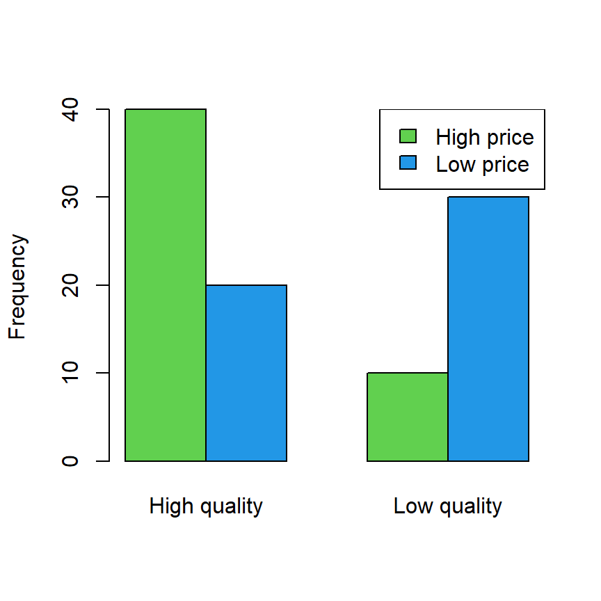
Now, if you want to check if quality and prices are independent you can perform a Chi-squared test passing the table or matrix with the data to the chisq.test function.
# Sample data
data <- matrix(c(40, 20, 10, 30), nrow = 2)
rownames(data) <- c("High price", "Low price")
colnames(data) <- c("High quality", "Low quality")

# Chi-squared test for independence
chi <- chisq.test(data)
chi
Pearson's Chi-squared test with Yates' continuity correction
data: data
X-squared = 15.042, df = 1, p-value = 0.0001052The p-value is almost zero, so there’s significant evidence to reject the null hypothesis that there is no association between the variables being tested. Therefore, there’s likely an association between quality and price.
Note that you can also return the expected counts and the Pearson’s residuals:
# Expected frequencies under H0
chi$expected

#            High quality Low quality
# High price           30          20
# Low price            30          20

# Pearson residuals
chi$residuals

#            High quality Low quality
# High price     1.825742   -2.236068
# Low price     -1.825742    2.236068

# Standardized residuals
chi$stdres

#            High quality Low quality
# High price     4.082483   -4.082483
# Low price     -4.082483    4.082483
You might have noticed that the previous test was conducted with the Yates’ continuity correction. Set correct = FALSE to avoid applying this correction.
It is recommended to use the Fisher’s exact test (fisher.test()) for 2x2 contingency tables instead of the Chi-squared test when the sample size is small (\(n < 30\)) or when the expected frequencies are lower than 5.
Chi-squared test for goodness-of-fit
This test examines whether an observed frequency distribution matches an expected theoretical distribution, such as a uniform distribution or any other expected distribution. This test expands the one-proportion Z-test.
The hypotheses are the following:
- \(H_0\): the distribution of the population IS F.
- \(H_1\): the distribution of the population IS NOT F.
If you have a vector with observed frequencies you can perform a chi-squared test to check if the observed frequencies fit the expected (theoretical) probabilities:
observed <- c(11, 32, 24)    # Observed frequencies
expected <- c(0.2, 0.5, 0.3) # Expected probabilities (sum up to 1)

# Chi-squared test for goodness of fit (Are the population probabilities equal to 'p'?)
chisq.test(x = observed, p = expected)
Chi-squared test for given probabilities
data: observed
X-squared = 1.2537, df = 2, p-value = 0.5343The p-value is greater than the usual significance levels, so there is no evidence to reject the null hypothesis.
Notice that you can also input expected frequencies instead of probabilities if you set rescale.p = TRUE, as the frequencies will be rescaled if necessary to sum to 1.
observed <- c(11, 32, 24) # Observed frequencies
expected <- c(20, 53, 25) # Expected frequencies

# Chi-squared test for goodness of fit with rescaled 'p'
chisq.test(x = observed, p = expected, rescale.p = TRUE)
Finally, if p is not specified, then the test will check whether the proportions are all equal (uniform distribution).
observed <- c(15, 25, 20)

# Are the population probabilities equal? (Is the population uniform?)
chisq.test(observed)
Chi-squared test for given probabilities
data: observed
X-squared = 2.5, df = 2, p-value = 0.2865The test returns a p-value of 0.2865, greater than the usual significance levels. Therefore, there is no statistical evidence to reject the null hypothesis of equal probabilities.
Chi-squared test of homogeneity
This test compares the distributions of a single categorical variable among several independent groups or populations. It determines whether the distribution of frequencies of a single categorical variable is similar or homogeneous across different groups. This test expands the two proportions Z-test.
The hypotheses are the following:
- \(H_0\): the distributions of two or more subgroups of a population ARE equal (equal proportions).
- \(H_1\): the distributions of two or more subgroups of a population ARE DIFFERENT (at least one proportion is different).
Chi-squared test of independence and chi-squared test of homogeneity are mathematically equal, but differ in a matter of design. While the independence test examines the relationship between two categorical variables in a single population, the test of homogeneity assesses whether the distribution of a categorical variable is homogeneous or consistent across different populations or groups.
Consider that you want to check if the distribution of frequencies of a treatment is equal or different across age groups (this is, if the proportion of usage of several drugs is equal or different among age groups):
| Drug A | Drug B | Drug C | |
|---|---|---|---|
| Age under 30 | 18 | 26 | 44 |
| Age over 30 | 6 | 14 | 19 |
The previous data can be created and represented in R with the following code:
# Sample data
data <- matrix(c(18, 26, 44, 6, 14, 19), nrow = 2, byrow = TRUE)
colnames(data) <- c("Drug A", "Drug B", "Drug C")
rownames(data) <- c("Age under 30", "Age over 30")

# Bar chart
barplot(data, beside = TRUE, col = 2:3,
        xlab = "Treatment", ylab = "Frequency")
legend("topleft", rownames(data), fill = 2:3)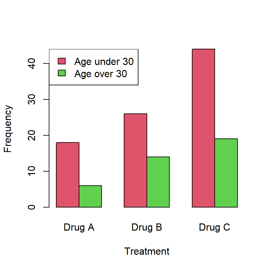
Now, you can perform a chi-squared test as illustrated below:
# Sample data
data <- matrix(c(18, 26, 44, 6, 14, 19), nrow = 2, byrow = TRUE)
colnames(data) <- c("Drug A", "Drug B", "Drug C")
rownames(data) <- c("Age under 30", "Age over 30")

# Chi-squared test of homogeneity
chisq.test(data)
Pearson's Chi-squared test
data: data
X-squared = 0.72271, df = 2, p-value = 0.6967The p-value is 0.6967, greater than the usual significance levels, so there is no evidence to reject the null hypothesis that the distribution is equal among the age groups.
When necessary, recall to set simulate.p.value = TRUE to compute p-values by Monte Carlo simulation with B replicates (by default B = 2000).