Tables in R with table() and prop.table()
The table function can be used for summarizing categorical data and generating absolute frequency and contigency tables. In this tutorial we will be exploring its syntax, various arguments, and practical examples to illustrate its utility in analyzing data. We will also explore the prop.table for relative frequency tables, xtabs for cross-tabulation, and addmargins to add margins to tables.
The table function
The table function in R is used to tabulate categorical data, counting the number of occurrences of each category. This function can create one-way tables, which provide the frequency of each category in a single variable, and two-way tables (or higher in high-dimensional arrays), which display the frequency distribution across two or more variables.
Syntax of the table function
The syntax of the function is the following:
table(...,
      exclude = if (useNA == "no") c(NA, NaN),
      useNA = c("no", "ifany", "always"),
      dnn = list.names(...),
      deparse.level = 1)
Being:
-
...: one or more categorical variables or expressions to be tabulated. -
exclude: optional argument specifying levels to be excluded from the table. -
useNA: treatment of missing values. Possible options are"no"(default),"ifany"and"always" -
dnn: character vector providing names for the resulting table. -
deparse.level: controls howdnnis constructed by default. Read the documentation of the function for additional details.
One-way frequency tables
One-way tables represent the frequency distribution of a single variable. They are useful for understanding the distribution of categories within a variable. In order to create a table you will need to input a character vector, as illustrated below:
# Sample data
data <- c("B", "A", "C", "C", "A", "C", "B")

# Create a simple frequency table for a categorical variable
one_way_table <- table(data)
one_way_table
data
A B C
2 2 3 The previous ouput means that there are two elements that correspond to category "A", two correspond to "B" and three to "C". The previous table can be represented using a bar plot:
# Sample data
data <- c("B", "A", "C", "C", "A", "C", "B")

# Create a simple frequency table for a categorical variable
one_way_table <- table(data)

# Plot the table
barplot(one_way_table, col = 2:4, ylab = "Count")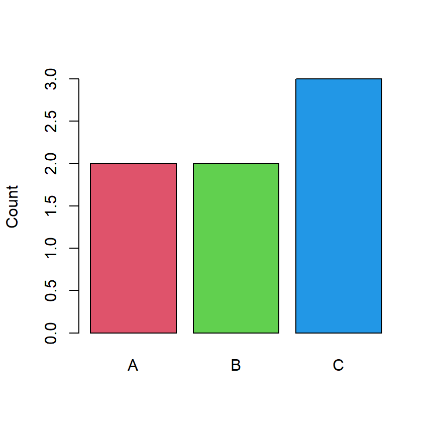
The function provides an argument named exclude that can be used to exclude some categories from the output table. In the following example we are excluding "B".
# Sample data
data <- c("B", "A", "C", "C", "A", "C", "B")

# Exclude specific levels from the frequency table
table(data, exclude = "B")
data
A C
2 3Sometimes, analyzing the presence of missing values is as important as the available data. The useNA argument can be leveraged to include NA values in the table. When set to "ifany" the table will also count the number of missing values.
# Sample data
data <- c("B", "A", NA, NA, "A", "C", "B")

# Count NA values if any
table(data, useNA = "ifany")
data
A B C <NA>
2 2 1 2 When set to "always" the table will display the number of NA values even if there were none. This is very useful for data checking.
# Sample data
data <- c("B", "A", "A", "C", "B")

# Count NA values even if there are none
table(data, useNA = "always")
data
A B C <NA>
2 2 1 0 Two-way contingency tables
Two-way tables show the relationship between two categorical variables. They are crucial for examining the interactions between variables. This type of table can also be created with the table function, but you will need to input two character vectors of the same length instead of one, as illustrated below.
# Sample data
gender <- c("Male", "Female", "Male", "Female", "Male")
age_group <- c("Junior", "Senior", "Senior", "Junior", "Junior")

# Create a two-way table
two_way_table <- table(gender, age_group)

# View the table
two_way_table
age_group
gender Junior Senior
Female 1 1
Male 2 1The previous data can be represented with a bar plot making use of the barplot function or any other similar function:
# Sample data
gender <- c("Male", "Female", "Male", "Female", "Male", "Female")
age_group <- c("Junior", "Senior", "Senior", "Junior", "Junior", "Senior")

# Create a two-way table
two_way_table <- table(gender, age_group)

# Plot the table
barplot(two_way_table, col = 2:3, beside = TRUE, ylab = "Count")
legend("topright", legend = c("Female", "Male"), fill = 2:3)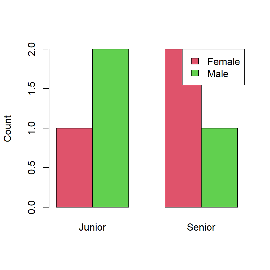
The prop.table function
The prop.table function takes a table created with table and converts it into a relative frequency table, also known as proportion table.
# Sample data
gender <- c("Male", "Female", "Male", "Female", "Male")
age_group <- c("Junior", "Senior", "Senior", "Junior", "Junior")

# Create a two-way table
two_way_table <- table(gender, age_group)

# Relative frequency table
prop.table(two_way_table)
age_group
gender Junior Senior
Female 0.2 0.2
Male 0.4 0.2The function includes an argument named margin. Setting margin to 1 calculates proportions based on the sum of each row, whereas setting it to 2 calculates proportions based on the sum of each column.
# Sample data
gender <- c("Male", "Female", "Male", "Female", "Male")
age_group <- c("Junior", "Senior", "Senior", "Junior", "Junior")

# Create a two-way table
two_way_table <- table(gender, age_group)

# Relative frequency table
prop.table(two_way_table, margin = 1)
age_group
gender Junior Senior
Female 0.5000000 0.5000000
Male 0.6666667 0.3333333
The xtabs function
A function related to table is xtabs. The xtabs function allows creating contingency tables and it is specially useful for grouped data and when working with data frames. Unlike table, it uses a formula syntax, which allows for more complex specifications and is ideal for statistical analysis.
# Sample data frame
df <- data.frame(x = c("G1", "G2", "G2", "G1", "G1", "G2"),
                 y = c("A", "B", "B", "C", "A", "C"))

# Contingency table with xtabs
tab <- xtabs(~ x + y, data = df)
tab
y
x A B C
G1 2 0 1
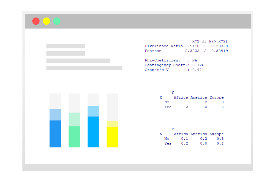
G2 0 2 1An interesting feature of xtabs is that it can create weighted contingency tables. The following example illustrates how to input weights using the column w:
# Sample data frame
df <- data.frame(x = c("G1", "G2", "G2", "G1", "G1", "G2"),
                 y = c("A", "B", "B", "C", "A", "C"),
                 w = c(0.1, 0.2, 0.2, 0.1, 0.1, 0.3))

# Weighted contingency table
tab <- xtabs(w ~ x + y, data = df)
tab
y
x A B C
G1 0.2 0.0 0.1
G2 0.0 0.4 0.3
The addmargins function
The addmargins function in R is used to add row and/or column margins, usually representing sums or totals of the rows and/or columns to tables created with table or similar functions. The syntax of the function is the following:
addmargins(A, margin = NULL, FUN = sum, quiet = FALSE)Being:
-
A: the input table. -
margin: the desired margin. By default, the function calculates all margins, but when is set to 1, only row margins are calculated, and when set to 2, only column margins are calculated. -
FUN: function to be applied to calculate the margins. It sums by default. -
quiet: logical. If set toTRUEsuppress messages.
When the function is applied to a table both margins will be added by default, counting the number of elements for rows and columns.
# Sample data
gender <- c("Male", "Female", "Male", "Female", "Male")
age_group <- c("Junior", "Senior", "Senior", "Junior", "Junior")

# Create a two-way table
two_way_table <- table(gender, age_group)

# Add margins
addmargins(two_way_table)
age_group
gender Junior Senior Sum
Female 1 1 2
Male 2 1 3
Sum 3 2 5However, if you only want to calculate the margins for rows or for columns you will need to set the margin argument to 1 or 2 depending on your needs.
# Sample data
gender <- c("Male", "Female", "Male", "Female", "Male")
age_group <- c("Junior", "Senior", "Senior", "Junior", "Junior")

# Create a two-way table
two_way_table <- table(gender, age_group)

# Add margins
addmargins(two_way_table, margin = 2)
age_group
gender Junior Senior Sum
Female 1 1 2
Male 2 1 3R version 4.3.2 (2023-10-31 ucrt)