Lilliefors normality test in R

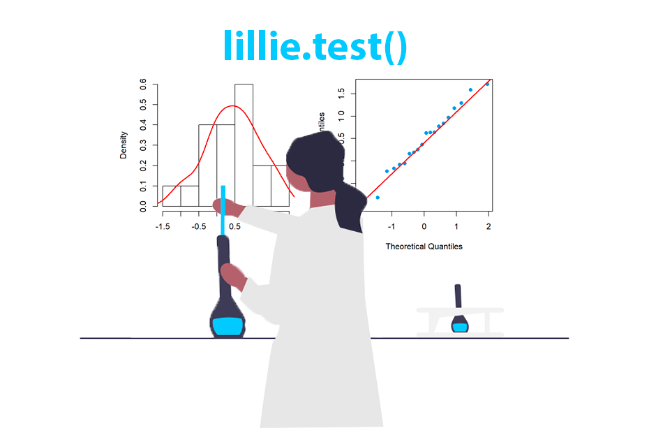
The lillie.test function is part of the nortest package and is used to conduct the Lilliefors test, which is a modified version of the Kolmogorov-Smirnov test for normality.

Hypothesis

The Lilliefors test is a variant of the Kolmogorov-Smirnov test that is specifically designed to test normality. It evaluates whether the data comes from a normal distribution by comparing the empirical distribution function of the data with the expected normal cumulative distribution function.

The null hypothesis of this test is that the distribution of the population is normal while the alternative hypothesis is that the distribution of the population is not normal:

• \(H_0\): the distribution of the population IS normal.
• \(H_1\): the distribution of the population is NOT normal.

Examples and interpretation

Sample normal data

For this example, let’s generate a sample dataset drawn from a normal distribution. The data can be visually examined using a histogram or a normal Q-Q plot to assess its normality:

# Sample data
set.seed(17)
x <- rnorm(20)

# One row, two columns plot
par(mfrow = c(1, 2))

# Histogram and density
hist(x, freq = FALSE, col = "white")
lines(density(x), lwd = 2, col = "red")

# QQ-plot
qqnorm(x, pch = 16, col = 4)
qqline(x, col = "red", lwd = 2)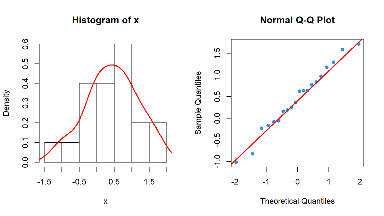

Now, a Lilliefors test can be conducted with the lillie.test function from nortest package to evaluate whether the population distribution of variable x follows a normal distribution:

# Sample data
set.seed(17)
x <- rnorm(20)

# install.packages("nortest")
library(nortest)

# Does 'x' follow a normal distribution?
lillie.test(x)

	Lilliefors (Kolmogorov-Smirnov) normality test

data:  x
D = 0.098636, p-value = 0.8775

The p-value of 0.8775 suggests there is no significant statistical evidence to reject the null hypothesis, indicating that the population likely conforms to a normal distribution.

Sample non-normal data

For this example we are going to use data drawn from an exponential distribution to check how the test performs:

# Sample data
set.seed(17)
x <- rexp(20)

# One row, two columns plot
par(mfrow = c(1, 2))

# Histogram and density
hist(x, freq = FALSE, col = "white")
lines(density(x), lwd = 2, col = "red")

# QQ-plot
qqnorm(x, pch = 16, col = 4)
qqline(x, col = "red", lwd = 2)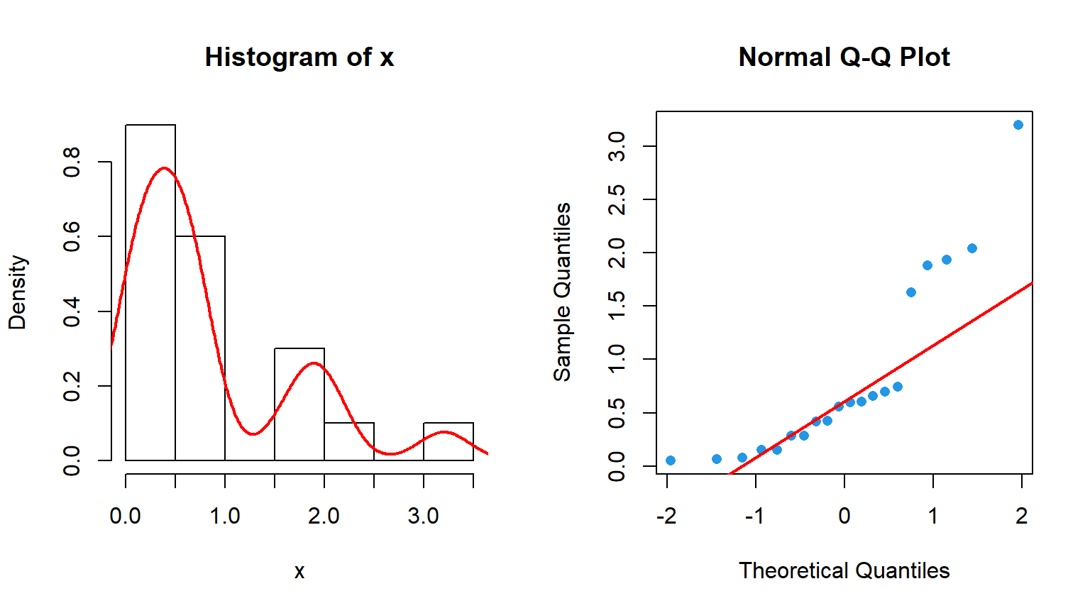

With a visual inspection of the data it is possible to see that the data might not follow a normal distribution. The Lilliefors test can be performed to check it:

# Sample data
set.seed(17)
x <- rexp(20)

# install.packages("nortest")
library(nortest)

# Does 'x' follow a normal distribution?
lillie.test(x)

	Lilliefors (Kolmogorov-Smirnov) normality test

data:  x
D = 0.28833, p-value = 0.0001262

In this scenario, the p-value is lower than the usual significance levels (0.1, 0.05 and 0.01) so there is strong evidence against the null hypothesis of normal distributed data.