Kolmogorov-Smirnov test in R with ks.test()

The Kolmogorov-Smirnov test (KS test) is a generic test used to compare the empirical distribution of data against a theoretical distribution or to test if two samples follow the same distribution. R provides a function named ks.test to perform this test.

Syntax of ks.test

The syntax of the ks.test function is the following:

ks.test(x, y, ...,
        alternative = c("two.sided", "less", "greater"),
        exact = NULL, simulate.p.value = FALSE, B = 2000)

Being:

• x: a numeric vector of values.
• y: for a two-sample test, the second numeric vector of data. For a one sample test, a string containing a cumulative distribution function ("pnorm", "punif", "pexp", …).
• alternative: the alternative hypothesis. Possible values are "two.sided" (default), "less" (the CDF of x is lower than the CDF of y) and "greater" (the CDF of x is greater than the CDF of y).
• exact: whether to compute exact p-values. Possible values are TRUE, FALSE and NULL (the default, which calculates exact p-values in some scenarios).
• simulate.p.value: if TRUE computes p-values by Monte Carlo simulation. Defaults to FALSE.
• B: number of replicates of Monte Carlo simulation. Defaults to 2000.

One sample KS test

The one-sample Kolmogorov-Smirnov (KS) test is a non-parametric statistical method used to determine if a single sample of data follows a specified continuous distribution (e.g., normal, exponential, etc.) or if it significantly differs from that distribution.

Let F be a continuous distribution, the null and alternative hypothesis for the Kolmogorov-Smirnov test for a single sample are the following:

• \(H_0\): the distribution of a population IS F.
• \(H_1\): the distribution of a population IS NOT F.

In the example below we compare the empirical distribution function of a variable named x against the theoretical cumulative distribution function of the standardized normal distribution. The objective is to check if the distribution of the population is normal.

# Sample data
set.seed(27)
x <- rnorm(50)

# Grid of values
grid <- seq(-4, 4, length.out = 100)

# Plot of CDFs
plot(grid, pnorm(grid, mean = 0, sd = 1), type = "l",
     ylim = c(0, 1), ylab = "", lwd = 2, col = "red", xlab = "", main = "ECDFs")
lines(ecdf(x), verticals = TRUE, do.points = FALSE, col.01line = NULL)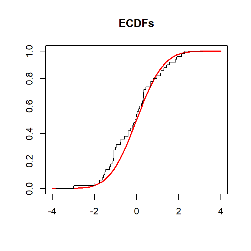

To perform the test you will have to input the data and the name of the cumulative distribution function (such as pnorm for normal distribution ,punif for uniform distribution, pexp for exponential distribution, …) and the desired parameters of the distribution.

# Sample data following a normal distribution
set.seed(27)
x <- rnorm(50)

# Does 'x' come from a standard normal distribution?
ks.test(x, "pnorm", mean = 0, sd = 1)

	Exact one-sample Kolmogorov-Smirnov test

data:  x
D = 0.083818, p-value = 0.8449
alternative hypothesis: two-sided

The p-value of the previous test is 0.8449, greater than the usual significance levels, implying there is no evidence to reject the null hypothesis that the distribution of the data is normal.

Now, we will perform the test again, but we will have a variable named y drawn from a normal distribution to be tested against a uniform distribution in the interval (-4, 4). In this scenario the cumulative distribution functions are the following:

# Sample data
set.seed(27)
y <- rnorm(50)

# Grid of values
grid <- seq(-5, 5, length.out = 100)

# Plot of CDFs
plot(grid, punif(grid, min = -4, max = 4), type = "l",
     ylim = c(0, 1), ylab = "", lwd = 2, col = "red", xlab = "", main = "ECDFs")
lines(ecdf(y), verticals = TRUE, do.points = FALSE, col.01line = NULL)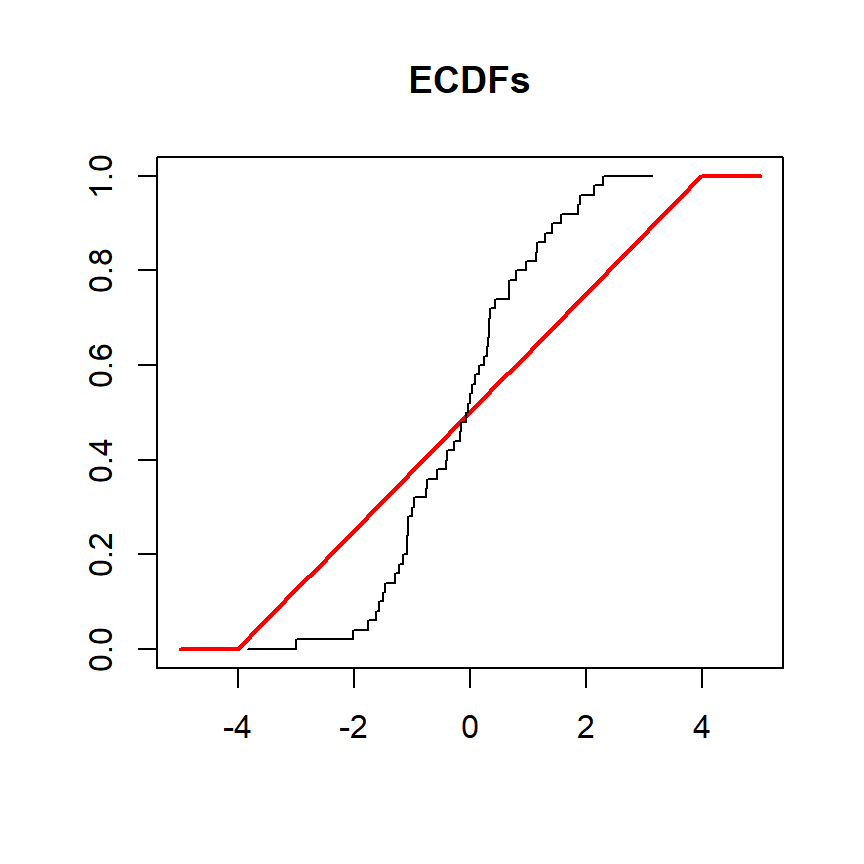

The test can be performed as shown in the example below:

# Sample data following a normal distribution
set.seed(27)
y <- rnorm(50)

# Does 'y' come from a uniform distribution in the interval (-4, 4)?
ks.test(y, "punif", min = -4, max = 4)

	Exact one-sample Kolmogorov-Smirnov test

data:  y
D = 0.23968, p-value = 0.005178
alternative hypothesis: two-sided

The test returns a p-value close to zero, which means there is statistical evidence to reject the null hypothesis that the data follows a uniform distribution.

Two sample KS test

The two-sample Kolmogorov-Smirnov (KS) test is a non-parametric method used to compare the empirical cumulative distribution functions (ECDFs) of two independent samples to determine if they are drawn from the same underlying distribution.

Let X and Y be two random independent variables the null and alternative hypotheses are the following:

• \(H_0\): the distribution of X IS EQUAL to the distribution of Y.
• \(H_1\): the distribution of X IS DIFFERENT to the distribution of Y.

The following block of code illustrates how to plot the cumulative distribution functions of two variables named x and y:

# Sample data
set.seed(27)
x <- runif(50, min = -1, max = 1)
y <- runif(50, min = -1, max = 1)

# Plot of CDFs
plot(ecdf(x), verticals = TRUE, do.points = FALSE, col.01line = NULL, xlab = "", main = "ECDFs")
lines(ecdf(y), verticals = TRUE, do.points = FALSE, col.01line = NULL, col = 4)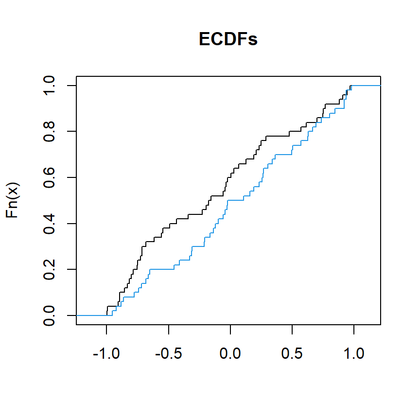

We can use ks.test to compare x and y to assess if they come from the same distribution.

# Sample data following a uniform distribution
set.seed(27)
x <- runif(50, min = -1, max = 1)
y <- runif(50, min = -1, max = 1)

# Two sample Kolmogorov-Smirnov test
# Does 'x' and 'y' come from the same distribution?
ks.test(x, y)

	Asymptotic two-sample Kolmogorov-Smirnov test

data:  x and y
D = 0.2, p-value = 0.2719
alternative hypothesis: two-sided

The p-value is 0.2719, greater than the usual significance levels, so there is no evidence to reject the null hypothesis. This means that there is not enough statistical evidence to conclude that the distributions of the two samples (x and y) are significantly different from each other.