Normal distribution in R
The Normal or Gaussian distribution is the most known and important distribution in Statistics. In this tutorial you will learn what are and what does dnorm, pnorm, qnorm and rnorm functions in R and the differences between them. In consequence, you will learn how to create and plot the Normal distribution in R, calculate probabilities under the curves, the quantiles, Normal random sampling and even how to shade a specific area under a Normal curve.
The normal or gaussian distribution
Among continuous random variables, the most important is the Normal or Gaussian distribution. This variable was introduced by Carl Friedrich in the XIX century for studying error measures.
Let \(X \sim N \left( \mu, \sigma \right)\), namely a random variable following a normal distribution with mean \(\mu\) and standard deviation \(\sigma\):
- The probability density function (PDF), also known as Bell curve, of \(x\) is \(f(x) = \frac{1}{\sqrt{2\pi \sigma^{2}}} e^{\frac{1}{2} (\frac{x - \mu}{\sigma})^2}\).
- The cumulative distribution function (CDF) is \(F(x) = P(X \leq x)\).
- The quantile function is \(Q(p) = F^{-1}(p)\).
- The expected mean and variance are \(E(X) = \mu\) and \(Var(X) = \sigma^2\), respectively.
In R there exist the dnorm, pnorm and qnorm functions, which allows calculating the normal density, distribution and quantile function for a set of values. In addition, the rnorm function allows obtaining random observations that follow a normal distibution. The following table summarizes the functions related to the normal distribution:
| Function | Description |
|---|---|
| dnorm |
Normal density (Probability Density Function) |
| pnorm |
Normal distribution (Cumulative Distribution Function) |
| qnorm | Quantile function of the Normal distribution |
| rnorm | Normal random number generation |
By default, these functions consider the standard Normal distribution, which has a mean of zero and a standard deviation of one.
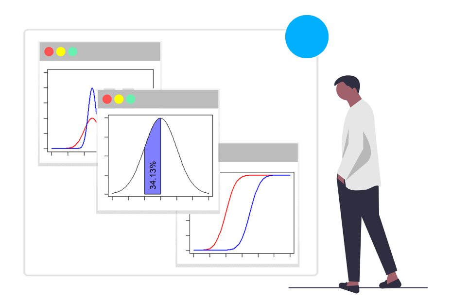
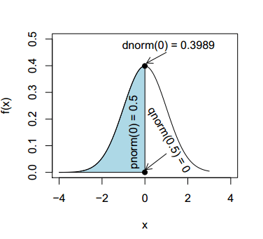
Although we will review each function in detail on the corresponding section, in the following illustration you can appreciate the relationship between the dnorm, pnorm and qnorm functions.
The dnorm function
In R, you can make use of the dnorm function to calculate the density function with mean \(\mu\) and standard deviation \(\sigma\) for any value of \(x, \mu\) and \(\sigma\).
dnorm(x,           # X-axis values (grid)
      mean = 0,    # Integer or vector representing the mean/s
      sd = 1,      # Integer or vector representing the standard deviation/s
      log = FALSE) # If TRUE, probabilities are given as log
Consider, for instance, that you want to obtain the PDF for \(x \in (-4, 4)\), with mean 1 and standard deviation of 3. In order to calculate it, you could type:
x <- -4:4
# x <- seq(-4, 4, length = 100) # More data points
dnorm(x, mean = 1, sd = 3)
0.03315905 0.05467002 0.08065691 0.10648267 0.12579441
0.13298076 0.12579441 0.10648267 0.08065691You can also specify vectors to the mean and sd arguments of the function. In the following example, the value of even elements are from \(\mu = 1, \sigma = 3\) and odds are from \(\mu = 2, \sigma = 4\).
dnorm(x, mean = c(1, 2), sd = c(3, 4))0.03315905 0.04566227 0.08065691 0.07528436 0.12579441
0.09666703 0.12579441 0.09666703 0.08065691Plot Normal distribution in R
Creating a normal distribution plot in R is easy. You just need to create a grid for the X-axis for the first argument of the plot function and pass as input of the second the dnorm function for the corresponding grid. In the following example we show how to plot normal distributions for different means and variances.
par(mfrow = c(1, 2))

# Grid of X-axis values
x <- seq(-4, 8, 0.1)

#-----------------------------------------
# Same standard deviation, different mean
#-----------------------------------------
# Mean 0, sd 1
plot(x, dnorm(x, mean = 0, sd = 1), type = "l",
     ylim = c(0, 0.6), ylab = "", lwd = 2, col = "red")
# Mean 3, sd 1
lines(x, dnorm(x, mean = 3, sd = 1), col = "blue", lty = 1, lwd = 2)

# Adding a legend
legend("topright", legend = c("0 1", "3 1"), col = c("red", "blue"),
       title = expression(paste(mu, " ", sigma)),
       title.adj = 0.9, lty = 1, lwd = 2, box.lty = 0)

#-----------------------------------------
# Same mean, different standard deviation
#-----------------------------------------
# Mean 1, sd 1
plot(x, dnorm(x, mean = 1, sd = 1), type = "l",
     ylim = c(0, 1), ylab = "", lwd = 2, col = "red")
# Mean 1, sd 0.5
lines(x, dnorm(x, mean = 1, sd = 0.5), col = "blue", lty = 1, lwd = 2)

# Adding a legend
legend("topright", legend = c("1 1", "1 0.5"), col = c("red", "blue"),
       title = expression(paste(mu, " ", sigma)),
       title.adj = 0.75, lty = 1, lwd = 2, box.lty = 0)

par(mfrow = c(1, 1))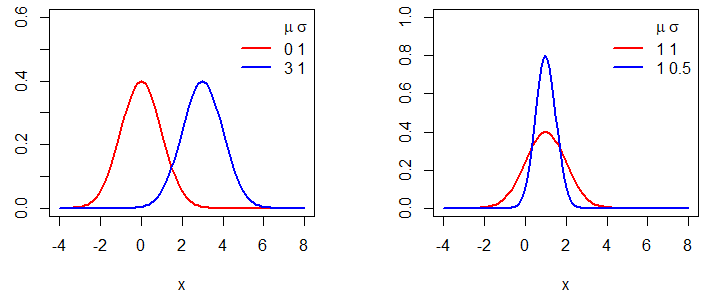
The pnorm function
The pnorm function gives the Cumulative Distribution Function (CDF) of the Normal distribution in R, which is the probability that the variable \(X\) takes a value lower or equal to \(x\).
The syntax of the function is the following:
pnorm(q,
      mean = 0,
      sd = 1,
      lower.tail = TRUE, # If TRUE, probabilities are P(X <= x), or P(X > x) otherwise
      log.p = FALSE)     # If TRUE, probabilities are given as log
As an example, taking into account that the Normal distribution is symmetric, the probability that the variable will take a value lower than the mean is 0.5:
pnorm(0, mean = 0, sd = 1) # 0.5pnorm function example
Now, suppose that you have a machine that packages rice inside boxes. The process follows a Normal distribution and it is known that the mean of the weight of each box is 1000 grams and the standard deviation is 10 grams. You can plot the density function typing:
Mean <- 1000
Sd <- 10

# X grid for non-standard normal distribution
x <- seq(-3, 3, length = 100) * Sd + Mean

# Density function
f <- dnorm(x, Mean, Sd)

plot(x, f, type = "l", lwd = 2, col = "blue", ylab = "", xlab = "Weight")
abline(v = Mean) # Vertical line on the mean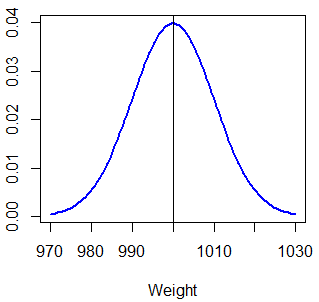
First, if you want to calculate the probability of a box weighing less than 1010 grams (\(P(X < 1010) = P(X \leq 1010)\)), you can type the following:
pnorm(1010, Mean, Sd) # 0.8413447 or 84.13%
1 - pnorm(1010, Mean, Sd, lower.tail = FALSE) # Equivalent
So the probability of a box weighting less than 1010 grams is 0.8413 or 84.13%, which corresponds to the following area:
lb <- min(x) # Lower bound
ub <- 1010   # Upper bound

x2 <- seq(min(x), ub, length = 100) # New Grid
y <- dnorm(x2, Mean, Sd) # Density

plot(x, f, type = "l", lwd = 2, col = "blue", ylab = "", xlab = "Weight")
abline(v = ub)

polygon(c(lb, x2, ub), c(0, y, 0), col = rgb(0, 0, 1, alpha = 0.5))
text(995, 0.01, "84.13%")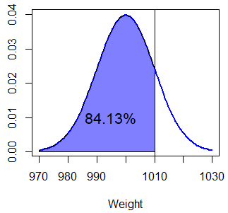
As shading the area under the Normal curve can be tricky and requires several lines of code, we have created a simple function to achieve it in a single line:
# mean: mean of the Normal variable
# sd: standard deviation of the Normal variable
# lb: lower bound of the area
# ub: upper bound of the area
# acolor: color of the area
# ...: additional arguments to be passed to lines function

normal_area <- function(mean = 0, sd = 1, lb, ub, acolor = "lightgray", ...) {
    x <- seq(mean - 3 * sd, mean + 3 * sd, length = 100)

    if (missing(lb)) {
       lb <- min(x)
    }
    if (missing(ub)) {
        ub <- max(x)
    }

    x2 <- seq(lb, ub, length = 100)
    plot(x, dnorm(x, mean, sd), type = "n", ylab = "")

    y <- dnorm(x2, mean, sd)
    polygon(c(lb, x2, ub), c(0, y, 0), col = acolor)
    lines(x, dnorm(x, mean, sd), type = "l", ...)
}
As an example, if you want to shade the area between -1 and 2 of a standard Normal distribution you can type:
normal_area(mean = 0, sd = 1, lb = -1, ub = 2, lwd = 2)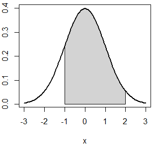
Second, in case that you want to calculate the probability of a box weighing more than 980 grams (\(P(X > 980) = P(X \geq 980)\)) you can use the lower.tail argument.
pnorm(980, Mean, Sd, lower.tail = FALSE) # 0.9772499 or 97.72%
1 - pnorm(980, Mean, Sd) # Equivalent
pnorm(1020, Mean, Sd)    # Equivalent by symmetry
The calculated probability corresponds to the following area:
normal_area(mean = Mean, sd = Sd, lb = 980, acolor = rgb(0, 0, 1, alpha = 0.5))
text(1000, 0.01, "97.72%")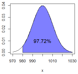
Finally, if you want to calculate the probability of a box weighing more than 990 grams and less than 1000 you have to calculate \(P(X \leq 1000) - P(x \leq 990) = P(X < 1000) - P(x <990)\) and hence you can type:
pnorm(1000, Mean, Sd) - pnorm(990, Mean, Sd) # 0.3413447 or 34.13%You can plot the area with the following code:
normal_area(mean = Mean, sd = Sd, lb = 990, ub = 1000,
            acolor = rgb(0, 0, 1, alpha = 0.5))
text(995, 0.01, "34.13%", srt = 90)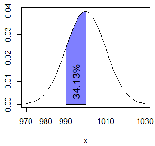
For continuous variables, as \(P(X = x) = 0\), \(P(X \geq x) = P(X > x)\) and \(P(X \leq x) = P(X < x)\).
Plot normal cumulative distribution function in R
With the pnorm function you can also plot the cumulative density function of the Gaussian or Normal distribution in R:
par(mfrow = c(1, 2))

# Grid of X-axis values
x <- seq(-4, 8, 0.1)

#-----------------------------------------
# Same standard deviation, different mean
#-----------------------------------------
# Mean 0, sd 1
plot(x, pnorm(x, mean = 0, sd = 1), type = "l",
     ylim = c(0, 1), ylab = "", lwd = 2, col = "red")
# Mean 3, sd 1
lines(x, pnorm(x, mean = 3, sd = 1), col = "blue", lty = 1, lwd = 2)

# Legend
legend("topleft", legend = c("0 1", "3 1"), col = c("red", "blue"),
       title = expression(paste(mu, " ", sigma)),
       title.adj = 0.9, lty = 1, lwd = 2, box.lty = 0)

#-----------------------------------------
# Same mean, different standard deviation
#-----------------------------------------
# Mean 1, sd 1
plot(x, pnorm(x, mean = 1, sd = 1), type = "l",
     ylim = c(0, 1), ylab = "", lwd = 2, col = "red")
# Mean 1, sd 0.5
lines(x, pnorm(x, mean = 1, sd = 0.5), col = "blue", lty = 1, lwd = 2)

# Legend
legend("topleft", legend = c("1 1", "1 0.5"), col = c("red", "blue"),
       title = expression(paste(mu, " ", sigma)),
       title.adj = 0.75, lty = 1, lwd = 2, box.lty = 0)

par(mfrow = c(1, 1))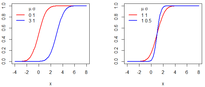
Recall that \(P(X < 0) = 0.5\) for a standard Normal distribution:
x <- seq(-4, 4, 0.1)
plot(x, pnorm(x, mean = 0, sd = 1), type = "l",
     ylim = c(0, 1), ylab = "P(X < x)", lwd = 2, col = "red")
segments(0, 0, 0, 0.5, lwd = 2, lty = 2)
segments(-4, 0.5, 0, 0.5, lwd = 2, lty = 2)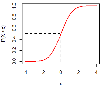
The qnorm function
The qnorm function allows you to find the quantile (percentile) \(Q\) for any probability \(p\). Hence, the qnorm function is the inverse of the pnorm function. The syntax of qnorm is as follows:
qnorm(p,                  # Integer or vector of probabilities
      mean = 0,           # Integer or vector of means
      sd = 1,             # Integer or vector of standard deviations
      lower.tail = TRUE,  # If TRUE, probabilities are P(X <= x), or P(X > x) otherwise
      log.p = FALSE)      # If TRUE, probabilities are given as log
As a first example, the quantile for probability 0.5 (\(Q(0.5)\)) on a symmetric distribution is equal to the mean:
qnorm(0.5, mean = 0, sd = 1) # 0In addition, you can obtain the quantile for any given probability. Note the relation between pnorm and qnorm functions:
x <- pnorm(-1.5, mean = 0, sd = 1) # 0.0668072
qnorm(x, mean = 0, sd = 1) # -1.5

normal_area(mean = 0, sd = 1, ub = -1.5,
            lwd = 2, acolor = rgb(0, 0, 1, alpha = 0.5))
arrows(-0.5, 0.1, -1.45, 0, lwd = 2, length = 0.2)
text(-0.25, 0.13, "-1.5", cex = 1.5)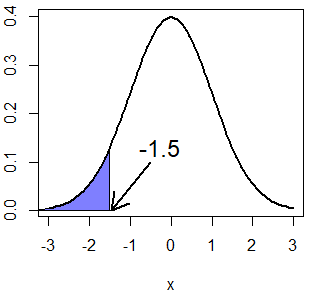
If you want to calculate, for instance, the quantile \(Q(P(X > 1.5)) = Q(1 - P(X \leq 1.5)) = Q(0.067)\) you can set the lower.tail argument to TRUE.
x <- pnorm(1.5, mean = 0, sd = 1, lower.tail = FALSE) # 0.0668072
qnorm(x, mean = 0, sd = 1, lower.tail = FALSE) # 1.5

# Equivalent to:
# x <- 1- pnorm(1.5, mean = 0, sd = 1)
# qnorm(1 - x, mean = 0, sd = 1)

normal_area(mean = 0, sd = 1, lb = 1.5, lwd = 2,
            acolor = rgb(0, 0, 1, alpha = 0.5))
arrows(0, 0.1, 1.45, 0, lwd = 2, length = 0.2)
text(0, 0.13, "1.5", cex = 1.5)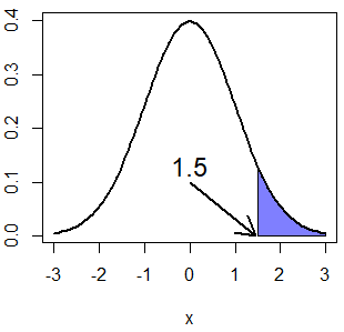
Plotting the Normal quantile function
You can plot the quantile function of a standard Normal distribution typing the following:
plot(qnorm, pnorm(-4), pnorm(4), lwd = 2, xlab = "p", ylab = "Q(p)")

# Equivalent to:
# x <- seq(pnorm(-4), pnorm(4), length = 100)
# plot(x, qnorm(x, mean = 0, sd = 1), type = "l",
#      lwd = 2, xlab = "p", ylab = "Q(p)")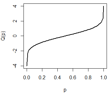
The previous plot represents the possible outcomes of the qnorm function for the standard Normal distribution. Recall that \(Q(0.5) = 0\):
plot(qnorm, pnorm(-4), pnorm(4), lwd = 2,
     xlab = "p", ylab = "Q(p)")
segments(0.5, -4, 0.5, 0, lty = 2, lwd = 2)
segments(0, 0, 0.5, 0, lty = 2, lwd = 2)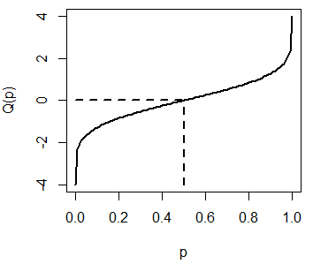
The rnorm function
The rnorm function generates \(n\) observations from the Normal distribution with mean \(\mu\) and standard deviation \(\sigma\). The syntax of the rnorm function in R is the following:
rnorm(n,        # Number of observations to be generated
      mean = 0, # Integer or vector of means
      sd = 1)   # Integer or vector of standard deviations
Hence, you can generate 10 observations of a standard Normal distribution in R with the following code:
rnorm(10)0.3320065 -0.6454991 -0.3692699 -0.4160260 0.5756340
-0.8793241 -0.8095590 0.4926698 -0.8038873 -0.3446890However, it should be noted that if you don’t specify a seed the output won’t be reproducible. You can make use of the set.seed function to make your code reproducible:
# Seed for reproducibility
set.seed(1)
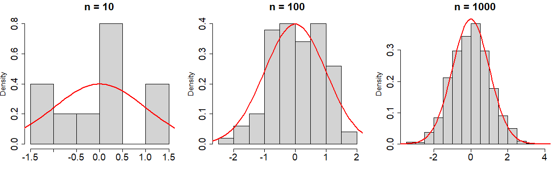
rnorm(1) # -0.6264538In addition, in the following plot you can observe how increasing the number of observations, the histogram of the data approaches to the true Normal density function:
par(mfrow = c(1, 3))

x <- seq(-10, 10, length = 200)

set.seed(3)
# n = 10
hist(rnorm(10, mean = 0, sd = 1), main = "n = 10",
     xlab = "", prob = TRUE)
lines(x, dnorm(x), col = "red", lwd = 2)

# n = 100
hist(rnorm(100, mean = 0, sd = 1), main = "n = 100",
     xlab = "", prob = TRUE)
lines(x, dnorm(x), col = "red", lwd = 2)

# n = 1000
hist(rnorm(1000, mean = 0, sd = 1), main = "n = 1000",
     xlab = "", prob = TRUE)
lines(x, dnorm(x), col = "red", lwd = 2)

par(mfrow = c(1, 1))