Calculate the median in R
The median is a measure of central tendency which can be defines as the value that divides a set of observations, ordered from lowest to highest into two parts with the same number of observations, or as the value which divides the data into two parts of equal probability. In this tutorial we will review how to calculate the median in R for both discrete and continuous variables, as well as calculate the median by groups.
Median of a discrete variable
To calculate the median of a set of observations we can use the median function. Consider the following vector:
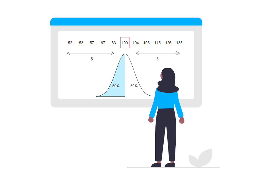
data <- c(126, 52, 133, 104, 115, 67, 57, 83, 53, 105, 100)In this case we can see that the median of the data is 100:
median(data) # 100We can check this by sorting the data and seeing that there is the same number of observations at both sides of the median. In this case there are 5 observations on the left and 5 observations on the right.
plot(1, 1, type = "n", axes = FALSE, ann = FALSE,
     xlim = c(0, 11), ylim = c(0, 1))
text(c(1:11), rep(0.5, 10), as.character(sort(data)))
rect(xleft = 5.6, ybottom = 0.45, xright = 6.4, ytop = 0.55, border = 2)
arrows(x0 = 0.7, y0 = 0.4, x1 = 5, code = 3, length = 0.15)
arrows(x0 = 7, y0 = 0.4, x1 = 11, code = 3, length = 0.15)
text(c(3, 9), 0.35, "5")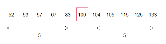
Note that if the number of observations is odd, the median will be calculated as the average of the two central values. Consider the same data as before except for the last observation:
data2 <- c(126, 52, 133, 104, 115, 67, 57, 83, 53, 105)In this case the median is 93.5:
median(data2) # 93.5The median corresponds to the average of the values 83 and 104, leaving 4 observations on each side, as illustrated in the following figure:
plot(1, 1, type = "n", axes = T, ann = FALSE,
     xlim = c(0, 11), ylim = c(0, 1))
text(c(1:10), rep(0.5, 10), as.character(sort(data2)))
rect(xleft = 4.5, ybottom = 0.45, xright = 6.5, ytop = 0.55, border = 2)
arrows(x0 = 0.7, y0 = 0.4, x1 = 4.25, code = 3, length = 0.15)
arrows(x0 = 6.75, y0 = 0.4, x1 = 10.5, code = 3, length = 0.15)
text(c(2.5, 8.5), 0.35, "4")
text(5.5, 0.6, "mean(c(83, 104)) = 93.5")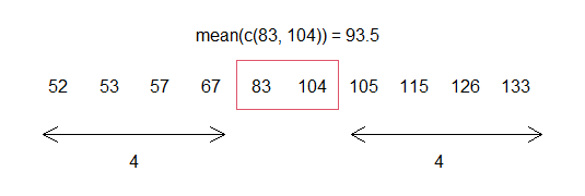
If the variable contains NA values you can set the argument na.rm to TRUE to delete them.
Median of a continuous variable
If instead of a discrete variable we have a continuous variable we can also use the median function. Consider a random sample of 1000 values drawn from a normal distribution with mean 0 and standard deviation 1:
set.seed(1)
data3 <- rnorm(1000)
In this case, we see that the median is very close to its theoretical value (as the normal distribution is symmetric, the mean and median are equal, so the theoretical median is 0). Recall that the median is the value that leaves a 50% probability or observations on both sides.
median(data3) # -0.03532423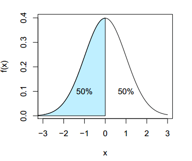
Median by groups in R
Finally, if we have a data set classified by groups we can use the tapply function to calculate the median per group. Take the following data as an example:
set.seed(1)
x <- sample(1:1000, 100)
group <- sample(c("A", "B", "C"), 100, replace = TRUE)
data4 <- data.frame(x, group)

head(data4)
x group
1 836 B
2 679 A
3 129 A
4 930 C
5 509 C
6 471 CWe can apply the tapply function to the data frame in the following way:
tapply(data4$x, data4$group, median) A B C
543.0 524.0 525.5The output will return the median for each group.