Exponential distribution in R
The exponential distribution is a continuous probability distribution used to model the time or space between events in a Poisson process. In this tutorial you will learn how to use the dexp, pexp, qexp and rexp functions and the differences between them. Hence, you will learn how to calculate and plot the density and distribution functions, calculate probabilities, quantiles and generate random samples from an exponential distribution in R.
The exponential distribution
The exponential distribution is the probability distribution of the time or space between two events in a Poisson process, where the events occur continuously and independently at a constant rate \(\lambda\).
It is important to know the probability density function, the distribution function and the quantile function of the exponential distribution. Let \(X \sim Exp( \lambda )\), that is to say, a random variable with exponential distribution with rate \(\lambda\):
- The probability density function (PDF) of \(x\) is \(f(x) = \lambda e^{- \lambda x}\) if \(x \geq 0\) or \(0\) otherwise.
- The cumulative distribution function (CDF) is \(F(x) = P(X \leq x) = 1 - e^{-\lambda x}\) if \(x \geq 0\) or \(0\) otherwise.
- The quantile function is \(Q(p) = F^{-1}(p) = \frac{-ln (1 - p)}{\lambda}\).
- The expected mean and variance of \(X\) are \(E(X) = \frac{1}{\lambda}\) and \(Var(X) = \frac{(b-a)^2}{12}\), respectively.
In R, the previous functions can be calculated with the dexp, pexp and qexp functions. In addition, the rexp function allows obtaining random observations following an exponential distribution. The functions are described in the following table:
| Function | Description |
|---|---|
| dexp |
Exponential density (Probability density function) |
| pexp |
Exponential distribution (Cumulative distribution function) |
| qexp | Quantile function of the exponential distribution |
| rexp | Exponential random number generation |
By default, these functions consider the exponential distribution of rate \(\lambda = 1\).
You can see the relationship between the three first functions in the following plot for \(\lambda = 1\):
The dexp function
The function in R to calculate the density function for any rate \(\lambda\) is the dexp function, described below:
dexp(x,           # X-axis values (> 0)
     rate = 1,    # Vector of rates (lambdas)
     log = FALSE) # If TRUE, probabilities are given as log
As an example, if you want to calculate the exponential density function of rate 2 for a grid of values in R you can type:
# Grid of values
x <- seq(from = 0, to = 8, by = 0.01)

# Exponential PDF of rate 2
dexp(x, rate = 2)
However, recall that the rate is not the expected value, so if you want to calculate, for instance, an exponential distribution in R with mean 10 you will need to calculate the corresponding rate:
# Exponential density function of mean 10
dexp(x, rate = 0.1) # E(X) = 1/lambda = 1/0.1 = 10
Plot exponential density in R
With the output of the dexp function you can plot the density of an exponential distribution. For that purpose, you need to pass the grid of the X axis as first argument of the plot function and the dexp as the second argument. In the following block of code we show you how to plot the density functions for \(\lambda = 1\) and \(\lambda = 2\).
# Grid of X-axis values
x <- seq(0, 8, 0.1)

# lambda = 2
plot(x, dexp(x, 2), type = "l",
     ylab = "", lwd = 2, col = "red")
# lambda = 1
lines(x, dexp(x, rate = 1), col = "blue", lty = 1, lwd = 2)

# Adding a legend
legend("topright", c(expression(paste(, lambda)), "2", "1"),
       lty = c(0, 1, 1), col = c("blue", "red"), box.lty = 0, lwd = 2)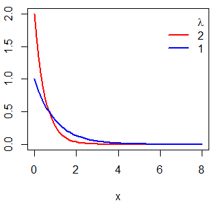
The pexp function
The R function that allows you to calculate the probabilities of a random variable \(X\) taking values lower than \(x\) is the pexp function, which has the following syntax:
pexp(q,
     rate = 1,
     lower.tail = TRUE, # If TRUE, probabilities are P(X <= x), or P(X > x) otherwise
     log.p = FALSE)
For instance, the probability of the variable (of rate 1) taking a value lower or equal to 2 is 0.8646647:
pexp(2) # 0.8646647pexp example: calculating exponential probabilities
The time spent on a determined web page is known to have an exponential distribution with an average of 5 minutes per visit. In consequence, as \(E(X) = \frac{1}{\lambda}\); \(5 = \frac{1}{\lambda}\); \(\lambda = 0.2\).
First, if you want to calculate the probability of a visitor spending up to 3 minutes on the site you can type:
pexp(3, rate = 0.2) # 0.4511884 or 45.12%
1 - pexp(3, rate = 0.2, lower.tail = FALSE) # Equivalent
In order to plot the area under an exponential curve with a single line of code you can use the following function that we have developed:
# rate: lambda parameter
# lb: lower bound of the area
# ub: upper bound of the area
# acolor: color of the area
# ...: additional arguments to be passed to the lines function
exp_area <- function(rate = 1, lb, ub, acolor = "lightgray", ...) {
    x <- seq(0, 12/rate, 0.01)

    if (missing(lb)) {
       lb <- min(x)
    }
    if (missing(ub)) {
        ub <- max(x)
    }

    x2 <- seq(lb, ub, length = 100)
    plot(x, dexp(x, rate = rate), type = "n", ylab = "")

    y <- dexp(x2, rate = rate)
    polygon(c(lb, x2, ub), c(0, y, 0), col = acolor)
    lines(x, dexp(x, rate = rate), type = "l", ...)
}
As an example, you could plot the area under an exponential curve of rate 0.5 between 0.5 and 5 with the following code:
exp_area(rate = 0.5, lb = 0.5, ub = 5, acolor = "white")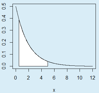
The calculated probability (45.12%) corresponds to the following area:
exp_area(rate = 0.2, ub = 3, acolor = rgb(0, 0, 1, alpha = 0.5))
text(1, 0.075, "45.12%", srt = 90, col = "white", cex = 1.2)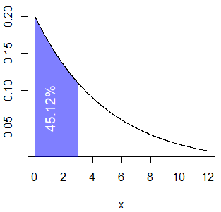
Second, if you want to calculate the probability of a visitor spending more than 10 minutes on the site you can type:
pexp(10, rate = 0.2, lower.tail = FALSE) # 0.1353353 or 13.53%The area that corresponds to the previous probability can be plotted with the following code:
exp_area(rate = 0.2, lb = 10, acolor = rgb(0, 0, 1, alpha = 0.5))
arrows(8, 0.1, 11, 0.015, length = 0.1, lwd = 2)
text(8, 0.12, "13.53%", cex = 1.2)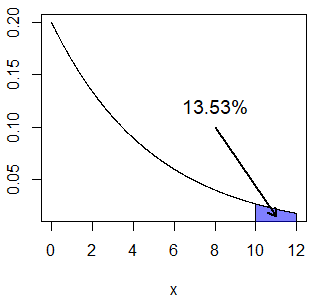
Finally, the probability of a visitor spending between 2 and 6 minutes is:
pexp(6, rate = 0.2) - pexp(2, rate = 0.2) # 0.3691258 or 36.91%The corresponding plot is the following:
exp_area(rate = 0.2, lb = 2, ub = 6, acolor = rgb(0, 0, 1, alpha = 0.5))
text(4, 0.05, "36.91%", col = "white", cex = 1.2)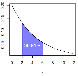
As the exponential distribution is a continuous distribution \(P(X = x) = 0\), so \(P(X \geq x) = P(X > x)\) and \(P(X \leq x) = P(X < x)\).
Plot exponential cumulative distribution function in R
You can plot the exponential cumulative distribution function passing the grid of values as first argument of the plot function and the output of the pexp function as the second.
# Grid of X-axis values
x <- seq(0, 12, 0.1)

# lambda = 2
plot(x, pexp(x, 2), type = "l",
     ylab = "F(x)", lwd = 2, col = "red")
# lambda = 1
lines(x, pexp(x, rate = 1), col = "blue", lty = 1, lwd = 2)

# Adding a legend
legend("topright", c(expression(paste(, lambda)), "1", "2"),
       lty = c(0, 1, 1), col = c("red", "blue"), box.lty = 0, lwd = 2)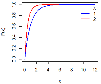
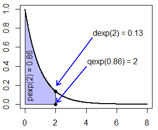
Recall that pexp(2) was equal to 0.8646647. In the following graph you can see the relationship between the distribution and the density function.
par(mfrow = c(1, 2))

#-----------------------------
# Distribution function
#-----------------------------
plot(x, pexp(x), type = "l", ylab = "F(x)", col = "blue", lwd = 2)
segments(2, 0, 2, pexp(2), lwd = 2, lty = 2)
segments(0, pexp(2), 2, pexp(2), lwd = 2, lty = 2)

#-----------------------------
# Probability density function
#-----------------------------
plot(x, dexp(x), type = "l", ylab = "f(x)", col = "red", lwd = 2)

# Area
exp_area(rate = 1, ub = 2, acolor = rgb(1, 0, 1, alpha = 0.1))
# Text
text(1, 0.1, "86.47%")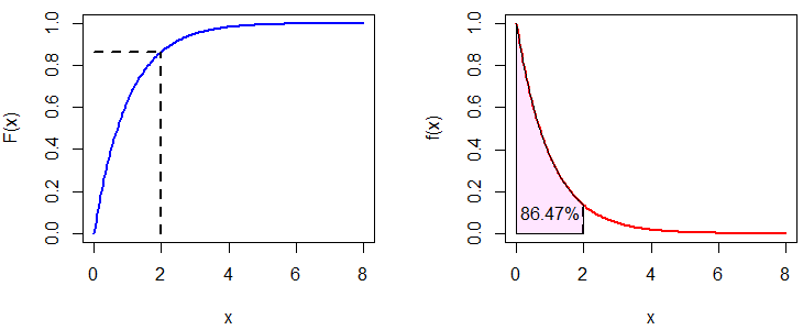
The qexp function
The qexp function allows you to calculate the corresponding quantile (percentile) for any probability \(p\):
qexp(q,
     rate = 1,
     lower.tail = TRUE, # If TRUE, probabilities are P(X <= x), or P(X > x) otherwise
     log.p = FALSE)
As an example, if you want to calculate the quantile for the probability 0.8646647 (\(Q(0.86)\)) you can type:
qexp(0.8646647) # 2
qexp(1 - 0.8646647, lower.tail = FALSE) # Equivalent
exp_area(rate = 1, ub = 2, acolor = rgb(0, 0, 1, alpha = 0.5))
points(2, 0, pch = 19)
arrows(4, 0.4, 2.2, 0.02, length = 0.1)
text(7.5, 0.5, "qexp(0.8646647) = 2", cex = 1.2)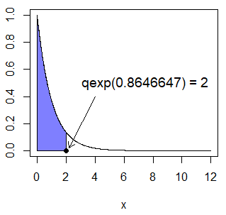
Recall that pexp(2) was equal to 0.8646647.
Set lower.tail = FALSE if you want the probability to be on the upper tail.
Plotting the exponential quantile function
You can make a plot of the exponential quantile function, which shows the possible outcomes of the qexp function, with the code of the following block:
plot(qexp, pexp(0), pexp(8), lwd = 2, xlab = "p", ylab = "Q(p)")
segments(0, 2, pexp(2), 2, lty = 2, lwd = 2)
segments(pexp(2), 0, pexp(2), qexp(0.8646647), lty = 2, lwd = 2)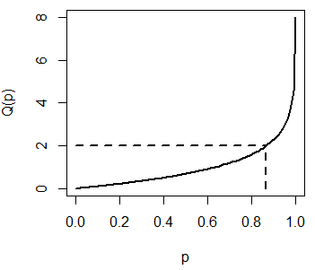
Recall that pexp(2) is equal to 0.8647 and qexp(0.8647) is equal to 2.
The rexp function
The rexp function allows you to draw \(n\) observations from an exponential distribution. The syntax of the function is as follows:
rexp(n, # Number of observations to be generated
     rate = 1)
As an example, if you want to draw ten observations from an exponential distribution of rate 1 you can type:
rexp(10)However, if you want to make the output reproducible you will need to set a seed for the R pseudorandom number generator:
set.seed(1)
rexp(10)
0.7551818 1.1816428 0.1457067 0.1397953 0.4360686
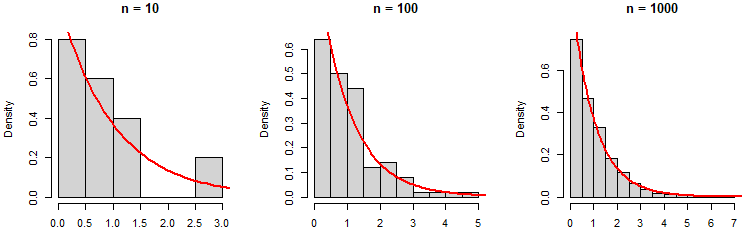
2.8949685 1.2295621 0.5396828 0.9565675 0.1470460Observe that as you increase the number of observations, the histogram of the data approaches to the true exponential density function:
# Three columns
par(mfrow = c(1, 3))

x <- seq(0, 12, length = 200)

set.seed(1)
# n = 10
hist(rexp(10), main = "n = 10",
     xlab = "", prob = TRUE)
lines(x, dexp(x), col = "red", lwd = 2)

# n = 100
hist(rexp(100), main = "n = 100",
     xlab = "", prob = TRUE)
lines(x, dexp(x), col = "red", lwd = 2)

# n = 1000
hist(rexp(1000), main = "n = 1000",
     xlab = "", prob = TRUE)
lines(x, dexp(x), col = "red", lwd = 2)

# Back to the original graphics device
par(mfrow = c(1, 1))