Continuous uniform distribution in R
The uniform distribution is a continuous distribution where all the intervals of the same length in the range of the distribution accumulate the same probability. In this tutorial we will explain how to use the dunif, punif, qunif and runif functions to calculate the density, cumulative distribution, the quantiles and generate random observations, respectively, from the uniform distribution in R.
Uniform distribution
Let \(X \sim U(a, b)\), this is, a random variable with uniform distribution in the interval \((a, b)\), with \(a, b \in \mathbb{R}, a < b\):
- The probability density function (PDF) of \(x\) is \(f(x) = \frac{1}{b - a}\) if \(x \in (a, b)\) and \(0\) otherwise.
- The cumulative distribution function (CDF) is \(F(x) = P(X \leq x) = \frac{x-a}{b-a}\).
- The quantile function is \(Q(p) = F^{-1}(p)\).
- The expected mean and variance of \(X\) are \(E(X) = \frac{a + b}{2}\) and \(Var(X) = \frac{(b-a)^2}{12}\), respectively.
The different functions of the uniform distribution can be calculated in R for any value of \(x\). These R functions are dunif, for the density function, punif, for the cumulative distribution and qunif, for the quantile function. Moreover, the runif function allows obtaining \(n\) random observations from the uniform distribution. These functions are described below:
| Function | Description |
|---|---|
| dunif |
Continuous uniform density (Probability density function) |
| punif |
Continuous uniform distribution (Cumulative distribution function) |
| qunif |
Quantile function of the uniform distribution |
| runif |
Random number generation of the uniform distribution |
By default, these functions consider the uniform distribution on the interval (0, 1), also known as standard uniform distribution.
The dunif function
In order to calculate the uniform density function in R in the interval \((a, b)\) for any value of \(x\) you can make use of the dunif function, which has the following syntax:
dunif(x,           # X-axis values (grid of values)
      min = 0,     # Lower limit of the distribution (a)
      max = 1,     # Upper limit of the distribution (b)
      log = FALSE) # If TRUE, probabilities are given as log
Consider that you want to calculate the uniform probability density function in the interval \((1, 3)\) for a grid of values. For that purpose you can type:
x <- 0:4 # Grid
dunif(x, min = 1, max = 3)
0.0 0.5 0.5 0.5 0.0Plot uniform density in R
You can plot the PDF of a uniform distribution with the following function:
# x: grid of X-axis values (optional)
# min: lower limit of the distribution (a)
# max: upper limit of the distribution (b)
# lwd: line width of the segments of the graph
# col: color of the segments and points of the graph
# ...: additional arguments to be passed to the plot function
plotunif <- function(x, min = 0, max = 1, lwd = 1, col = 1, ...) {

    # Grid of X-axis values
    if (missing(x)) {
        x <- seq(min - 0.5, max + 0.5, 0.01)
    }

    if(max < min) {
        stop("'min' must be lower than 'max'")
    }

    plot(x, dunif(x, min = min, max = max),
         xlim = c(min - 0.25, max + 0.25), type = "l",
         lty = 0, ylab = "f(x)", ...)
    segments(min, 1/(max - min), max, 1/(max - min), col = col, lwd = lwd)
    segments(min - 2, 0, min, 0, lwd = lwd, col = col)
    segments(max, 0, max + 2, 0, lwd = lwd, col = col)
    points(min, 1/(max - min), pch = 19, col = col)
    points(max, 1/(max - min), pch = 19, col = col)
    segments(min, 0, min, 1/(max - min), lty = 2, col = col, lwd = lwd)
    segments(max, 0, max, 1/(max - min), lty = 2, col = col, lwd = lwd)
    points(0, min, pch = 21, col = col, bg = "white")
    points(max, min, pch = 21, col = col, bg = "white")
}
As an example, if you want to plot the uniform density function in the interval (0, 1) in blue you can type:
plotunif(min = 0, max = 1, lwd = 2, col = 4, main = "Uniform PDF")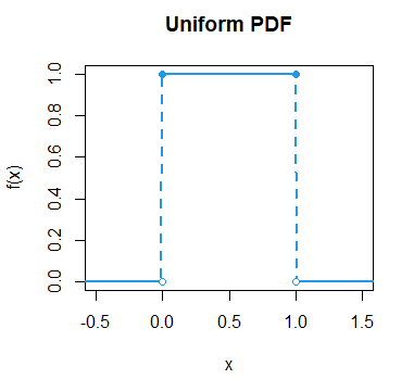
The punif function
In R, you can use the punif function to calculate the uniform cumulative distribution function, this is, the probability of a variable \(X\) taking a value lower than \(x\). This function has the following syntax:
punif(q,                  # Vector of quantiles
      min = 0,            # Lower limit of the distribution (a)
      max = 0,            # Upper limit of the distribution (b)
      lower.tail = TRUE,  # If TRUE, probabilities are P(X <= x), or P(X > x) otherwise
      log.p = FALSE)      # If TRUE, probabilities are given as log
As an example, if you want to calculate the probability of a uniform variable on the interval \((0, 1)\) taking a value equal or lower to 0.6 is:
punif(0.6) # 0.6punif function example
Consider, for instance, that \(X\) is the time (in minutes) that a person has to wait in order to take a flight. If each flight takes off each hour \(X \sim U(0, 60)\). Taking the latter into account:
- The probability of waiting less than 15 minutes is \(P(X < 15) = P(X \leq 15)\):
punif(15, min = 0, max = 60) # 0.25 or 25%
1 - punif(15, min = 0, max = 60, lower.tail = FALSE) # Equivalent
We have developed the following function to shade the area over an interval of the uniform probability density function with a single line of code:
# min: lower limit of the distribution (a)
# max: upper limit of the distribution (b)
# lb: lower bound of the area
# ub: upper bound of the area
# col: color of the lines and points
# acolor: color of the area
# ...: additional arguments to be passed to the plot function
unif_area <- function(min = 0, max = 1, lb, ub, col = 1,
                      acolor = "lightgray", ...) {
    x <- seq(min - 0.25 * max, max + 0.25 * max, 0.001)

    if (missing(lb)) {
       lb <- min(x)
    }
    if (missing(ub)) {
        ub <- max(x)
    }
    if(max < min) {
        stop("'min' must be lower than 'max'")
    }

    x2 <- seq(lb, ub, length = 1000)
    plot(x, dunif(x, min = min, max = max),
         xlim = c(min - 0.25 * max, max + 0.25 * max), type = "l",
         ylab = "f(x)", lty = 0, ...)

    y <- dunif(x2, min = min, max = max)
    polygon(c(lb, x2, ub), c(0, y, 0), col = acolor, lty = 0)
    segments(min, 1/(max - min), max, 1/(max - min), lwd = 2, col = col)
    segments(min - 2 * max, 0, min, 0, lwd = 2, col = col)
    segments(max, 0, max + 2 * max, 0, lwd = 2, col = col)
    points(min, 1/(max - min), pch = 19, col = col)
    points(max, 1/(max - min), pch = 19, col = col)
    segments(min, 0, min, 1/(max - min), lty = 2, col = col, lwd = 2)
    segments(max, 0, max, 1/(max - min), lty = 2, col = col, lwd = 2)
    points(0, min, pch = 21, col = col, bg = "white")
    points(max, min, pch = 21, col = col, bg = "white")
}
As an example, if you want to plot the area between 0 and 0.5 of a uniform distribution on the interval \((0, 1)\), which can be calculated with punif(0.5), you can type:
unif_area(min = 0, max = 1, lb = 0, ub = 0.5,
          main = "punif(0.5)", acolor = "white")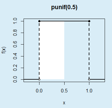
The calculated probability (0.25) corresponds to the following area:
unif_area(min = 0, max = 60, lb = 0, ub = 15)
text(8, 0.008, "25%", srt = 90, cex = 1.2)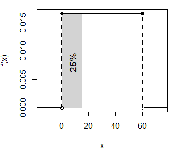
- The probability of waiting more than 45 minutes is \(P(X > 45) = 1 - P(X \leq 45)\):
punif(45, min = 0, max = 60, lower.tail = FALSE) # 0.25 or 25%
1 - punif(45, min = 0, max = 60) # Equivalent
That corresponds to:
unif_area(min = 0, max = 60, lb = 45, ub = 60)
text(51, 0.008, "25%", srt = 90, cex = 1.2)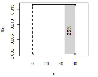
- The probability of waiting between 20 and 30 minutes is \(P(X \leq 30) - P(X \leq 20)\):
punif(30, min = 0, max = 60) - punif(20, min = 0, max = 60) # 0.167 or 16.7%The calculated probability can be represented with the following code:
unif_area(min = 0, max = 60, lb = 20, ub = 30)
text(24, 0.008, "16.7%", srt = 90, cex = 1.2)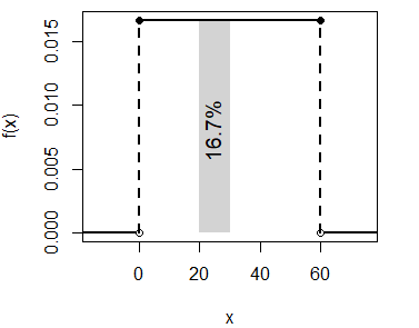
As the uniform distribution is a continuous distribution \(P(X = x) = 0\), so \(P(X \geq x) = P(X > x)\) and \(P(X \leq x) = P(X < x)\).
Plot uniform cumulative distribution
function in R
You can also plot the cumulative distribution function of the uniform distribution in R. You just need to type the following:
# Grid of X-axis values
x <- seq(-0.5, 1.5, 0.01)

# Uniform distribution between 0 and 1
plot(x, punif(x), type = "l", main = "Uniform CDF",
     ylab = "F(x)", lwd = 2, col = "red")

# Equivalent to:
plot(punif, -0.5, 1.5, type = "l", main = "Uniform CDF",
     ylab = "F(x)", lwd = 2, col = "red")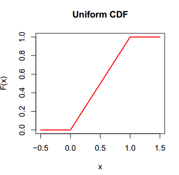
The qunif function
In R, you can calculate the corresponding quantile for any probability (p) for a uniform distribution with the qunif function, which has the following syntax:
qunif(p,                 # Vector of probabilities
      min = 0,           # Lower limit of the distribution (a)
      max = 1,           # Upper limit of the distribution (b)
      lower.tail = TRUE, # If TRUE, probabilities are P(X <= x), or P(X > x) otherwise
      log.p = FALSE)     # If TRUE, probabilities are given as log
In case you want to calculate the quantile for the probability 0.5 of a uniform distribution on the interval \((0, 60)\) you can type:
qunif(0.5, min = 0, max = 60) # 30unif_area(min = 0, max = 60, lb = 0, ub = 30)
text(15, 0.008, "50%", srt = 90, cex = 1.2)
arrows(38, 0.005, 31, 0.0005, length = 0.15)
text(44, 0.006, "qunif(0.5)")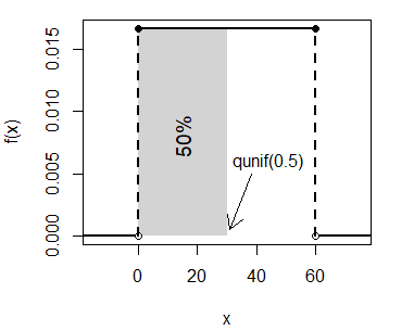
Plot of the uniform quantile function
It is possible to create the graph of a uniform quantile function in R. For that purpose you can type the following to plot the function on the interval \((0, 1)\):
plot(qunif, punif(0), punif(1), lwd = 2,
     main = "Uniform quantile function",
     xlab = "p", ylab = "Q(p)")
segments(0, 0.5, punif(0.5), 0.5, lty = 2, lwd = 2)
segments(punif(0.5), 0, punif(0.5), qunif(0.5), lty = 2, lwd = 2)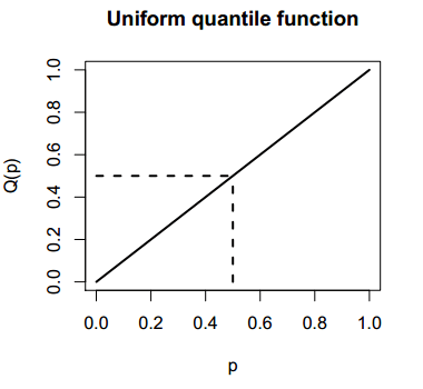
Recall that punif(0.5) = 0.5 and qunif(0.5) = 0.5.
The runif function
The R runif function allows drawing \(n\) random observations from a uniform distribution. The arguments of the function are described below:
runif(n        # Number of observations to be generated
      min = 0, # Lower limit of the distribution (a)
      max = 0) # Upper limit of the distribution (b)
As an example, you can draw ten observations from a uniform distribution on the interval \((-1, 1)\) typing:
runif(n = 10, min = -1, max = 1)-0.20757312 -0.46819001 -0.80643735 -0.92675885 0.80520074
0.39716130 -0.39939392 0.78837145 0.28130687 0.09807602However, every time you run the previous code you will obtain ten different numbers. If you want to make the output reproducible, you can set a seed with the set.seed function.
set.seed(1)
runif(n = 10, min = -1, max = 1)
-0.4689827 -0.2557522 0.1457067 0.8164156 -0.5966361
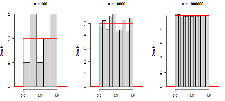
0.7967794 0.8893505 0.3215956 0.2582281 -0.8764275Observe that as we increase the number of generated observations, the histogram of the sampled data approaches to the true uniform density function:
# Three columns
par(mfrow = c(1, 3))

x <- seq(-0.5, 1.5, 0.01)

set.seed(1)

# n = 10
hist(runif(10), main = "n = 100", xlim = c(-0.2, 1.25),
     xlab = "", prob = TRUE)
lines(x, dunif(x), col = "red", lwd = 2)

# n = 1000
hist(runif(1000), main = "n = 10000", xlim = c(-0.2, 1.25),
     xlab = "", prob = TRUE)
lines(x, dunif(x), col = "red", lwd = 2)

# n = 100000
hist(runif(100000), main = "n = 1000000", xlim = c(-0.2, 1.25),
     xlab = "", prob = TRUE)
lines(x, dunif(x), col = "red", lwd = 2)

# Back to the original graphics device
par(mfrow = c(1, 1))