Box Cox transformation in R

The Box-Cox transformation is a power transformation that corrects asymmetry of a variable, different variances or non linearity between variables. In consequence, it is very useful to transform a variable and hence to obtain a new variable that follows a normal distribution.
Box cox family
The Box-Cox functions transformations are given for different values of \(\lambda\) by the following expression:
\[\begin{cases} \frac{x^{\lambda} - 1}{\lambda} \quad \text{ if } \quad \lambda \neq 0 \\log(x) \text{ if } \quad \lambda = 0\end{cases},\]
being \(y\) the variable to be transformed and \(\lambda\) the transformation parameter. However, the most common transformations are described in the following table:
| \(\lambda\) | Transformation |
|---|---|
| -2 | \(1/x^2\) |
| -1 | \(1/x\) |
| -0.5 | \(1/\sqrt{x}\) |
| 0 | \(\log(x)\) |
| 0.5 | \(\sqrt{x}\) |
| 1 | x |
| 2 | \(x^2\) |
If the estimated transformation parameter is close to one of the values of the previous table, in the practice it is recommended to pick up the value of the table instead of the exact value, as the value from the table is easier to interpret.
The boxcox function in R
When using R, we can make use of the boxcox function from the MASS package to estimate the transformation parameter by maximum likelihood estimation. This function will also give us the 95% confidence interval of the parameter. The arguments of the function are the following:
boxcox(object,    # lm or aov objects or formulas
       lambda = seq(-2, 2, 1/10), # Vector of values of lambda
       plotit = TRUE,  # Create a plot or not
       interp,         # Logical. Controls if spline interpolation is used
       eps = 1/50,     # Tolerance for lambda. Defaults to 0.02.
       xlab = expression(lambda), # X-axis title
       ylab = "log-Likelihood",   # Y-axis title
       …) # Additional arguments for model fitting
Box Cox transformation example
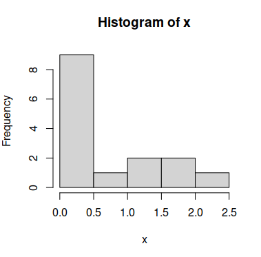
Consider the following sample vector x, which doesn’t follow a normal distribution:
x <- c(0.103, 0.528, 0.221, 0.260, 0.091,
            1.314, 1.732, 0.244, 1.981, 0.273,
            0.461, 0.366, 1.407, 0.079, 2.266)

# Histogram of the data
hist(x)
In order to calculate the optimal \(\lambda\) you have to compute a linear model with the lm function and pass it to the boxcox function as follows:
# install.packages(MASS)
library(MASS)

boxcox(lm(x ~ 1))
The output of the function will be the following plot:
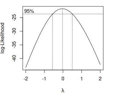
Note that the center dashed vertical line represents the estimated parameter \(\hat{\lambda}\) and the others the 95% confidence interval of the estimation.
As the previous plot shows that the 0 is inside the confidence interval of the optimal \(\lambda\) and as the estimation of the parameter is really close to 0 in this example, the best option is to apply the logarithmic transformation of the data (see the table of the first section).
# Transformed data
new_x <- log(x)

# Histogram
hist(new_x)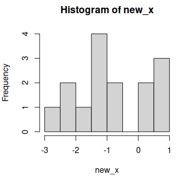
Now the data looks more like following a normal distribution, but you can also perform, for instance, a statistical test to check it, as the Shapiro-Wilk test:
shapiro.test(new.x)Shapiro-Wilk normality test
data: new_x
W = 0.9, p-value = 0.2As the p-value is greater than the usual levels of significance (1%, 5% and 10%) we have no evidence to reject the null hypothesis of normality.
Extracting the exact lambda
If the confidence interval of the estimated parameter doesn’t fit with any value of the table you can extract the exact lambda using the following code:
# install.packages(MASS)
library(MASS)

b <- boxcox(lm(x ~ 1))

# Exact lambda
lambda <- b$x[which.max(b$y)] # -0.02
Now you can make the transformation of the variable using the expression of the first section:
new_x_exact <- (x ^ lambda - 1) / lambda
new_x_exact