Poisson distribution in R
The Poisson distribution is a discrete distribution that counts the number of events in a Poisson process. In this tutorial we will review the dpois, ppois, qpois and rpois functions to work with the Poisson distribution in R.
The Poisson distribution
Denote a Poisson process as a random experiment that consist on observe the occurrence of specific events over a continuous support (generally the space or the time), such that the process is stable (the number of occurrences, \(\lambda\) is constant in the long run) and the events occur randomly and independently.
The Poisson distribution is used to model the number of events that occur in a Poisson process. Let \(X \sim P(\lambda)\), this is, a random variable with Poisson distribution where the mean number of events that occur at a given interval is \(\lambda\):
- The probability mass function (PMF) is \(P(X = x) =\frac{e^{- \lambda} \lambda^x}{x!}\) for \(x = 0, 1, 2, \dots\).
- The cumulative distribution function (CDF) is \(F(x) =\sum_{i = 0}^x \frac{e ^{- \lambda} \lambda^i}{i!}\).
- The quantile function is \(Q(p) = F ^{-1}(p)\).
- The expected mean and variance of \(X\) are \(E(X) = Var(X) = \lambda\).
The functions described in the list before can be computed in R for a set of values with the dpois (probability mass), ppois (distribution) and qpois (quantile) functions. Moreover, the rpois function allows obtaining \(n\) random observations that follow a Poisson distribution. The table below describes briefly each of these functions.
| Function | Description |
|---|---|
| dpois |
Poisson probability mass function (Probability function) |
| ppois |
Poisson distribution (Cumulative distribution function) |
| qpois | Poisson quantile function |
| rpois |
Poisson pseudorandom number generation |
The dpois function
The Poisson probability function with mean \(\lambda\) can be calculated with the R dpois function for any value of \(x\). The following block of code summarizes the arguments of the function:
dpois(x,           # X-axis values (x = 0, 1, 2, ...)
      lambda,      # Mean number of events that occur on the interval
      log = FALSE) # If TRUE, probabilities are given as log
As an example, if you want to calculate the Poisson mass probability function for \(x \in \{0, 1, \dots, 10\}\) with mean 5, you can type:
dpois(0:10, lambda = 5)0.006737947 0.033689735 0.084224337 0.140373896 0.175467370 0.175467370
0.146222808 0.104444863 0.065278039 0.036265577 0.018132789You can also specify a vector of means instead of a single value, as in the following block:
dpois(5, lambda = c(5, 10)) # 0.17546737 0.03783327In the previous example, the first element of the output is from a distribution with mean \(\lambda = 5\) and the second from a distribution with mean \(\lambda = 10\) events per interval.
Plot of the Poisson probability function in R
The Poisson probability mass function can be plotted in R making use of the plot function, as in the following example:
# Grid of X-axis values
x <- 0:50

#-----------
# lambda: 5
#-----------
lambda <- 5
plot(dpois(x, lambda), type = "h", lwd = 2,
     main = "Poisson probability function",
     ylab = "P(X = x)", xlab = "Number of events")

#-----------
# lambda: 10
#-----------
lambda <- 10
lines(dpois(x, lambda), type = "h", lwd = 2, col = rgb(1,0,0, 0.7))

#-----------
# lambda: 20
#-----------
lambda <- 20
lines(dpois(x, lambda), type = "h", lwd = 2, col = rgb(0, 1, 0, 0.7))

# Legend
legend("topright", legend = c("5", "10", "20"),
       title = expression(lambda), title.adj = 0.75,
       lty = 1, col = 1:3, lwd = 2, box.lty = 0)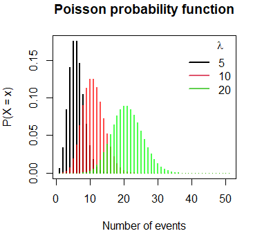
The ppois function
The probability of a variable \(X\) following a Poisson distribution taking values equal or lower than \(x\) can be calculated with the ppois function, which arguments are described below:
ppois(q,                 # Quantile or vector of quantiles
      lambda,            # Mean or vector of means
      lower.tail = TRUE, # If TRUE, probabilities are P(X <= x), or P(X > x) otherwise
      log.p = FALSE)     # If TRUE, probabilities are given as log
If you want to calculate, for instance, the probability of observing 5 or less events \((P(X \leq 5))\) if the mean of events occurring on a specific interval is 10 you can type:
ppois(5, lambda = 10) # 0.06708596In this example, the previous result is equivalent to the sum of the probabilities of each value up to 5:
sum(dpois(0:5, lambda = 10)) # 0.06708596ppois example
In this section we are going to present a more detailed example using the ppois function. Consider that the number of visits on a web page is known to follow a Poisson distribution with mean 15 visits per hour. Hence, \(\lambda = 15\).
- The probability of getting 10 or less visits per hour, \(P(X \leq 10)\), is:
ppois(10, lambda = 15) # 0.1184644 or 11.8%
1 - ppois(10, lambda = 15, lower.tail = FALSE) # Equivalent
sum(dpois(0:10, lambda = 15)) # Equivalent
As the Poisson distribution is discrete, the cumulative probability is calculated adding the corresponding probabilities of the probability function. The following R function allows to visualize the probabilities that are added based on a lower bound and an upper bound.
# lambda: mean
# lb: lower bound of the sum
# ub: upper bound of the sum
# col: color
# lwd: line width
pois_sum <- function(lambda, lb, ub, col = 4, lwd = 1, ...) {
    x <- 0:(lambda + lambda * 2)

    if (missing(lb)) {
       lb <- min(x)
    }
    if (missing(ub)) {
        ub <- max(x)
    }

    plot(dpois(x, lambda = lambda), type = "h", lwd = lwd, ...)

    if(lb == min(x) & ub == max(x)) {
        color <- col
    } else {
        color <- rep(1, length(x))
        color[(lb + 1):ub ] <- col
    }

    lines(dpois(x, lambda = lambda), type = "h",
          col =  color, lwd = lwd, ...)
}
By way of illustration, if you want to display the probabilities that have been added to calculate the probability of observing between 10 and 15 events, if 10 events occur on average on each interval, you can type:
 pois_sum(lambda = 10, lb = 10, ub = 15, lwd = 2,
           col = 2, ylab = "P(X = x)", xlab = "Number of events")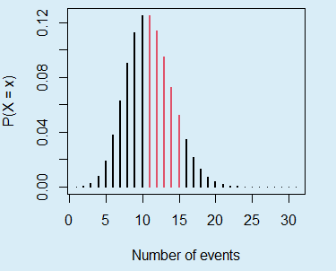
The sum of the probabilities displayed in red is equal to ppois(15, lambda = 10) - ppois(10, lambda = 10).
The calculated probability (11.8%) corresponds to the sum of the following probabilities:
pois_sum(lambda = 15, ub = 10, lwd = 2,
         ylab = "P(X = x)", xlab = "Visits per hour")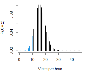
- The probability of getting more than 20 visits per hour, \(P(X > 20)\), is:
ppois(20, lambda = 15, lower.tail = FALSE) # 0.08297091 or 8.3%
1 - ppois(20, lambda = 15)        # Equivalent
1 - sum(dpois(0:20, lambda = 15)) # Equivalent
This probability corresponds to:
pois_sum(lambda = 15, lb = 20, lwd = 2,
         ylab = "P(X = x)", xlab = "Visits per hour")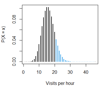
- The probability of getting less than 15 visits per hour, \(P(X < 15)\) is:
ppois(14, lambda = 15, lower.tail = FALSE) # 0.5343463 or 53.43%
1 - sum(dpois(0:15, lambda = 15)) # Equivalent
Note that we set 14 instead of 15, because the Poisson probability is discrete, so \(P(X < 15) =P(X \leq 14)\). The corresponding plot is as follows:
pois_sum(lambda = 15, ub = 14, lwd = 2,
         ylab = "P(X = x)", xlab = "Visits per hour")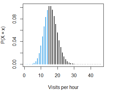
- The probability of receiving between 10 and 20 visits per hour is:
ppois(20, lambda = 15) - ppois(10, lambda = 15) # 0.7985647 or 79.86%
sum(dpois(11:20, lambda = 15)) # Equivalent
The probability can be represented making use of the function we defined before:
pois_sum(lambda = 15, lb = 10, ub = 20, lwd = 2,
         ylab = "P(X = x)", xlab = "Visits per hour")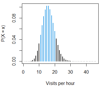
As the Poisson distribution is a discrete distribution \(P(X = x) \neq 0\), so \(P(X \geq x) \neq P(X > x)\) and \(P(X \leq x) \neq P(X < x)\).
Plot of the Poisson distribution function in R
The cumulative distribution of the Poisson distribution can be represented for different values of \(\lambda\) with the following block of code:
# Grid of X-axis values
x <- 0:50

#-----------
# lambda: 5
#-----------
lambda <- 5
plot(ppois(x, lambda), type = "s", lwd = 2,
     main = "Poisson distribution function",
     xlab = "Number of events", ylab = "F(x)")

#-----------
# lambda: 10
#-----------
lambda <- 10
lines(ppois(x, lambda), type = "s", lwd = 2, col = 2)

#-----------
# lambda: 20
#-----------
lambda <- 20
lines(ppois(x, lambda), type = "s", lwd = 2, col = 3)

# Legend
legend("bottomright", legend = c("5", "10", "20"),
       title = expression(lambda), title.adj = 0.75,
       lty = 1, col = 1:3, lwd = 2, box.lty = 0)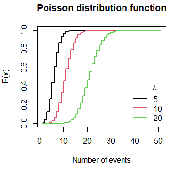
The qpois function
The R qpois function allows obtaining the corresponding Poisson quantiles for a set of probabilities.
qpois(p,                 # Probability or vector of probabilities
      lambda,            # Mean or vector of means
      lower.tail = TRUE, # If TRUE, probabilities are P(X <= x), or P(X > x) otherwise
      log.p = FALSE)     # If TRUE, probabilities are given as log
For instance, the quantile 0.5 of a Poisson distribution is equal to the mean:
qpois(0.5, lambda = 10) # 10Plot of the Poisson quantile function
The Poisson quantile function can be plotted in R for a set of probabilities. The following graph shows the outcomes of the qpois function for different means.
#-----------
# lambda: 20
#-----------
plot(qpois(seq(0, 1, 0.001), lambda = 20),
     main = "Poisson quantile functions",
     ylab = "Q(p)", xlab = "p",
     type = "s", col = 3, xaxt = "n")

axis(1, labels = seq(0, 1, 0.1), at = 0:10 * 100)

#-----------
# lambda: 10
#-----------
lines(qpois(seq(0, 1, 0.001), lambda = 10), type = "s", col = 2)

#-----------
# lambda: 5
#-----------
lines(qpois(seq(0, 1, 0.001), lambda = 5), type = "s")

# Legend
legend("topleft", legend = c("5", "10", "20"),
       title = expression(lambda), title.adj = 0.75,
       lty = 1, col = 1:3, lwd = 2, box.lty = 0)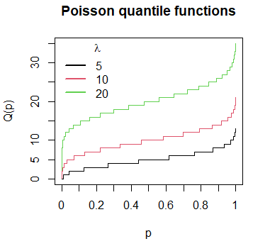
The rpois function
If you want to draw \(n\) observations from a Poisson distribution you can make use of the rpois function. The following block of code summarizes the arguments of the function.
rpois(n,      # Number of random observations to be generated
      lambda) # Mean or vector of means
If you want to obtain 10 random observations from a Poisson distribution with mean 4 in R you can type:
rpois(10, lambda = 4)7 6 2 2 3 6 3 4 4 7However, the previous output won’t be reproducible. In case you need to generate a reproducible sequence of numbers you can set a seed with any integer number as follows:
set.seed(10)
rpois(10, lambda = 4)
4 3 3 5 1 2 3 3 4 3