Mode estimation in R
The mode is a measure of location that can be defined as the most probable outcome of a random variable or as the most frequent value on a set of observations. It is a robust measure that coincides with the mean and the median in symmetric distributions. In this tutorial we will review how to calculate the mode in R for both discrete and continuous one-dimensional variables.
Discrete unimodal estimation
Consider the following vector x:
x <- c(1, 5, 1, 6, 2, 1, 6, 7, 1)The mode can be calculated as the most repeated value withing the variable, which in this case is 1. A simple way of calculating the mode in R in this case is using the following function:
mode <- function(x) {
   return(as.numeric(names(which.max(table(x)))))
}
In this case, we can check that the mode is 1 passing the vector to the function:
mode(x) # 1If you want to visualize the number of times that each data point is repeated you can also create a bar chart.
barplot(table(x), col = c(4, rep("gray", 4)))
legend("topright", "Mode", fill = 4)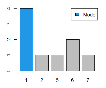
Continous unimodal estimation
If our variable of interest in continuous instead of discrete we cannot use the previous procedure, but we must resort to another method. The most usual procedure in the literature is calculating the maximum of the estimation of the density function of the data making use of any algorithm.
Consider the following normal data (unimodal) with mean 0 and standard deviation of 1. As the normal distribution is symmetric, we know that the mean, the median and the mode are equal (0).
set.seed(1234)
x2 <- rnorm(1000)
In order to visualize the modes you can draw the histogram and the density function estimation. Note that the the selection of the bandwidth will determine the shape of the estimated density.
# Histogram
hist(x2, freq = FALSE)
# Density
dx <- density(x2)
lines(dx$x, dx$y, col = 2, lwd = 2)
# Theoretical mode
abline(v = 0, col = 4, lty = 2, lwd = 3)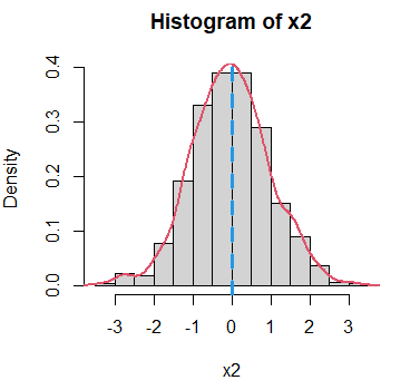
In order to perform the calculation you will need to use the mlv function of the modeest package, that allows selection among different algorithms. We recommend you to use the mean-shift algorithm, as displayed on the following block of code.
# install.packages("modeest")
library(modeest)

# Moda
mlv(x2, method = "meanshift") # -0.03912067
We can observe that the estimated mode (-0.039) is very close to the theoretical mode (0). Other available methods are “lientz”, “naive”, “venter”, “grenander”, “hsm”, “parzen”, “tsybakov” and “asselin”.
Discrete multimodal estimation
Unlike the median or mean, the mode can take multiple values at the same time. For instance, consider the vector y, which has two modes.
y <- c(3, 5, 3, 3, 5, 6, 5)

# Histogram
hist(y)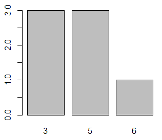
In this case the most repeated values are 3 and 5. In order to calculate several modes you can make use of the mlv function of the modeest package and apply the mfv method.
# install.packages("modeest")
library(modeest)

# Modes
mlv(y, method = "mfv") # 3 5
Continuous multimodal estimation
In you want to calculate several modes when our variable is continuous you can use the locmodes of the multimode package.
Consider the following multimodal data, which theoretical modes are 40 y 120, represented with vertical red lines.
n <- 1000
bin <- rbinom(n, 1, 0.6)
y2 <- rnorm(n, mean = 120, sd = 11) * bin +
      rnorm(n, mean = 40, sd = 5) * (1 - bin)

# Histogram
hist(y2)
# Theoretical mode 1
abline(v = 40, col = 2, lwd = 2)
# Theoretical mode 2
abline(v = 120, col = 2, lwd = 2)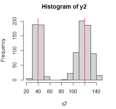
You can apply the locmodes function to the previous data, indicating the number of modes that you expect to find in the mod0 argument.
# install.packages("multimode")
library(multimode)

modes <- locmodes(y2, mod0 = 2)
modes
Estimated location
Modes: 40.56825 120.8625
Antimode: 69.94661
Estimated value of the density
Modes: 0.02535653 0.02033563
Antimode: 8.184294e-08
Critical bandwidth: 3.746696
Warning message:
In locmodes(y, mod0 = 2) :
If the density function has an unbounded support, artificial modes may have been created in the tailsOn the previous output you can observe that the estimated modes are 40.57 and 120.86, very close to the theoretical values.
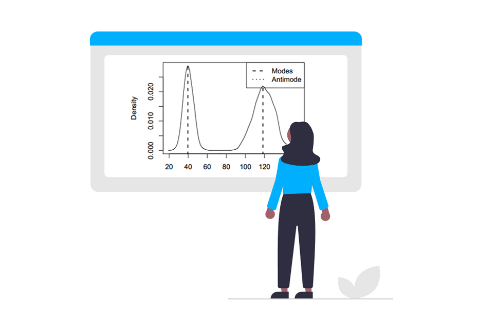
The library also provides a S3 method to plot the estimations returned by the locmodes function, displaying the localization of the modes, of the antimodes and the bandwidth used.
plot(modes)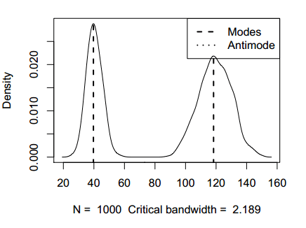
The package also provides the modetest function to test for multimodality and functions for exploring the number of modes, such as modetree, modeforest and sizes.