Covariance and correlation in R

The cor and cov functions are both useful to analyze relationships between variables, but while the first calculates the correlation coefficient, the second computes the covariance.

Syntax

The syntax of both functions is the same:

# Covariance
cov(x, y = NULL, use = "everything",
    method = c("pearson", "kendall", "spearman"))

# Correlation
cor(x, y = NULL, use = "everything",
    method = c("pearson", "kendall", "spearman"))

Being:

• x, y: vectors, data frames, or matrices containing numeric data.
• use: determines how to handle missing values. Default is "everything", but it can also be set to "complete.obs", "pairwise.complete.obs", or "na.or.complete".
• method: specifies the method to compute the correlation coefficient. Options include "pearson" (default), "kendall", or "spearman".

Covariance

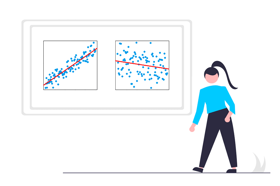
The covariance is a metric of joint variation that indicates if there is linear relationship between variables. This coefficient is usually denoted as \(S\) and the interpretation is the following:

• If \(S > 0\), implies a positive relationship.
• If \(S \approx 0\), there is no relationship.
• If \(S < 0\), implies a negative relationship.

In addition, the higher the covariance coefficient, the higher the relationship.

In R, the cov function can be used to calculate the covariance coefficient between two numeric vectors:

# Sample data
set.seed(15)
x <- rnorm(100)
y <- x + rnorm(100)

# Covariance coefficient between x and y
cov(x, y)

1.028619

The function returns a value of 1.028619, indicating a positive linear relationship between \(x\) and \(y\).

Covariance matrix

If the input of the function is a numeric matrix or data frame instead of two numeric vectors the function will compute the covariances between the columns of the dataset.

# Sample data
set.seed(15)
df <- data.frame(Var1 = rnorm(100), Var2 = runif(100), Var3 = rexp(100))

# Covariance matrix of 'df'
cov(df)

            Var1         Var2         Var3
Var1  0.98795201 -0.024517909 -0.079986687
Var2 -0.02451791  0.084020062 -0.009591341
Var3 -0.07998669 -0.009591341  2.118357213

You can also input two data frames or matrices to calculate the correlation between the columns of the datasets.

# Sample data
set.seed(15)
df <- data.frame(Var1 = rnorm(100), Var2 = runif(100), Var3 = rexp(100))
df2 <- data.frame(Var4 = rnorm(100), Var5 = runif(100), Var6 = rexp(100))

# Covariance matrix between 'df' and 'df2'
cov(df, df2)

             Var4         Var5        Var6
Var1 -0.001427763  0.014351821 -0.05569541
Var2  0.041006100  0.005160602 -0.06376888
Var3  0.064429874 -0.053229349  0.03178257

Correlation

The main problem of the covariance is that it is not bounded and it depends on the units of measure. In order to solve this issues, there is the correlation coefficient, usually denoted as \(r\), which is a dimensionless metric that ranges from -1 to 1.

• If \(r = 1\), implies there is a perfect positive relationship.
• If \(r > 0\), implies a positive relationship.
• If \(r \approx 0\), there is no correlation between variables.
• If \(r < 0\), implies a negative relationship.
• If \(r = - 1\), there is a perfect negative relationship.

The correlation coefficient can be calculated with the cor function.

Pearson correlation coefficient

The default correlation coefficient calculated by cor is named Pearson correlation coefficient. In the example below we are calculating the correlation coefficient for \(x\) and \(y\):

# Sample data
set.seed(15)
x <- rnorm(100)
y <- x + rnorm(100)

# Correlation coefficient between x and y
cor(x, y)

0.6856568

The function returns a coefficient of 0.6856568, indicating a strong positive relationship between the two variables.

Kendall’s tau correlation coefficient

The Kendall coefficient of correlation, also known as Kendall’s \(\tau\) is suitable for ordinal or non-normally distributed data, as it is based on the rank or order of values rather than the actual values. Set method = "kendall" to compute it.

# Sample data
set.seed(15)
x <- rnorm(100)
y <- x + rnorm(100)

# Kendall's correlation coefficient between x and y
cor(x, y, method = "kendall")

0.4840404

The function returns a coefficient of 0.4840404, implying a positive relationship between \(x\) and \(y\).

Spearman’s rho correlation coefficient

The Spearman’s correlation coefficient (Spearman’s \(\rho\)) is a robust and non-parametric alternative of the Pearson’s coefficient, also based on the rank of values as Kendall’s \(\tau\). It is commonly used when the data is not normal or has outliers, as it better captures possible nonlinear relationships between variables. Set method = "spearman" to calculate it.

# Sample data
set.seed(15)
x <- rnorm(100)
y <- x + rnorm(100)

# Spearman's correlation coefficient between x and y
cor(x, y, method = "spearman")

0.6706871

The function returns a coefficient of 0.6706871, very similar to Pearson’s coefficient, also indicating a strong positive relationship between the two variables.

Correlation matrix

If you input a data frame or matrix with several columns to cor it will compute the correlation matrix for the variables, as illustrated in the following example.

# Sample data
set.seed(15)
df <- data.frame(Var1 = rnorm(100), Var2 = runif(100), Var3 = rexp(100))

# Correlation matrix of 'df'
cor(df)

            Var1        Var2        Var3
Var1  1.00000000 -0.08509891 -0.05529046
Var2 -0.08509891  1.00000000 -0.02273465
Var3 -0.05529046 -0.02273465  1.00000000

You can also pass two data frames or matrices as input to compute the correlation between the columns of the first data set with the columns of the second.

# Sample data
set.seed(15)
df <- data.frame(Var1 = rnorm(100), Var2 = runif(100), Var3 = rexp(100))
df <- data.frame(Var1 = rnorm(100), Var2 = runif(100))

# Correlation matrix between 'df' and 'df2'
cor(df, df2)

            Var4        Var5        Var6
Var1  1.00000000 -0.03199334 -0.11915007
Var2 -0.03199334  1.00000000  0.04328424

Covariance to correlation matrix with cov2cor

R also provides an useful function named cov2cor that allows to transform a covariance matrix into a correlation matrix efficiently. The function takes a covariance matrix as input, as shown below.

# Sample data
set.seed(15)
df <- data.frame(Var1 = rnorm(100), Var2 = runif(100), Var3 = rexp(100))

# Covariance matrix of 'df'
S <- cov(df)

# Covariance to correlation matrix
cov2cor(S)

            Var1        Var2        Var3
Var1  1.00000000 -0.08509891 -0.05529046
Var2 -0.08509891  1.00000000 -0.02273465
Var3 -0.05529046 -0.02273465  1.00000000