Binomial distribution in R

The binomial distribution is a discrete distribution that counts the number of successes in Bernoulli experiments or trials. In this tutorial we will explain how to work with the binomial distribution in R with the dbinom, pbinom, qbinom, and rbinom functions and how to create the plots of the probability mass, distribution and quantile functions.
The binomial distribution
Denote a Bernoulli process as the repetition of a random experiment (a Bernoulli trial) where each independent observation is classified as success if the event occurs or failure otherwise and the proportion of successes in the population is constant and it doesn’t depend on its size.
Let \(X \sim B(n, p)\), this is, a random variable that follows a binomial distribution, being \(n\) the number of Bernoulli trials, \(p\) the probability of success and \(q = 1 - p\) the probability of failure:
- The probability mass function (PMF) is \(P(X = x) = \binom{n}{x}p^x q^{n-x}\) if \(x = 0, 1, 2, \dots, n\).
- The cumulative distribution function (CDF) is \(F(x) = I_q(1 - x, n-x)\).
- The quantile function is \(Q(p) = F^{-1}(p)\).
- The expected mean and variance of \(X\) are \(E(X) = np\) and \(Var(X) = npq\), respectively.
The functions of the previous lists can be computed in R for a set of values with the dbinom (probability), pbinom (distribution) and qbinom (quantile) functions. In addition, the rbinom function allows drawing \(n\) random samples from a binomial distribution in R. The following table describes briefly these R functions.
| Function | Description |
|---|---|
| dbinom |
Binomial probability mass function (Probability function) |
| pbinom |
Binomial distribution (Cumulative distribution function) |
| qbinom | Binomial quantile function |
| rbinom |
Binomial pseudorandom number generation |
In the following sections we will review each of these functions in detail.
The dbinom function
In order to calculate the binomial probability function for a set of values \(x\), a number of trials \(n\) and a probability of success \(p\) you can make use of the dbinom function, which has the following syntax:
dbinom(x,           # X-axis values (x = 0, 1, 2, ..., n)
       size,        # Number of trials (n > = 0)
       prob,        # The probability of success on each trial
       log = FALSE) # If TRUE, probabilities are given as log
For instance, if you want to calculate the binomial probability mass function for \(x = 1, 2, \dots, 10\) and a probability of success in each trial of 0.2, you can type:
dbinom(x = 1:10, size = 10, prob = 0.2)0.2684354560 0.3019898880 0.2013265920 0.0880803840 0.0264241152
0.0055050240 0.0007864320 0.0000737280 0.0000040960 0.0000001024Plot of the binomial probability function in R
The binomial probability mass function can be plotted in R making use of the plot function, passing the output of the dbinom function of a set of values to the first argument of the function and setting type = “h” as follows:
# Grid of X-axis values
x <- 1:80

# size = 80, prob = 0.2
plot(dbinom(x, size = 80, prob = 0.2), type = "h", lwd = 2,
     main = "Binomial probability function",
     ylab = "P(X = x)", xlab = "Number of successes")

# size = 80, prob = 0.3
lines(dbinom(x, size = 80, prob = 0.3), type = "h",
      lwd = 2, col = rgb(1,0,0, 0.7))

# size = 80, prob = 0.4
lines(dbinom(x, size = 80, prob = 0.4), type = "h",
      lwd = 2, col = rgb(0, 1, 0, 0.7))

# Add a legend
legend("topright", legend = c("80  0.2", "80  0.3", "80  0.4"),
       title = "size  prob", title.adj = 0.95,
       lty = 1, col = 1:3, lwd = 2, box.lty = 0)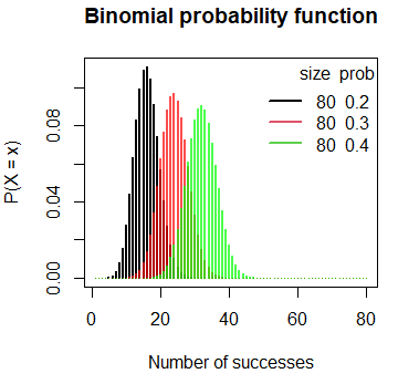
The pbinom function
In order to calculate the probability of a variable \(X\) following a binomial distribution taking values lower than or equal to \(x\) you can use the pbinom function, which arguments are described below:
pbinom(q,                 # Quantile or vector of quantiles
       size,              # Number of trials (n > = 0)
       prob,              # The probability of success on each trial
       lower.tail = TRUE, # If TRUE, probabilities are P(X <= x), or P(X > x) otherwise
       log.p = FALSE)     # If TRUE, probabilities are given as log
By ways of illustration, the probability of the success occurring less than 3 times if the number of trials is 10 and the probability of success is 0.3 is:
pbinom(3, size = 10, prob = 0.3) # 0.6496107 or 64.96%As the binomial distribution is discrete, the previous probability could also be calculated adding each value of the probability function up to three:
sum(dbinom(0:3, size = 10, prob = 0.3)) # 0.6496107 or 64.96%As the binomial distribution is discrete, the cumulative probability can be calculated adding the corresponding probabilities of the probability function. The following R function allows visualizing the probabilities that are added based on a lower bound and an upper bound.
# size: number of trials (n > = 0)
# prob: probability of success on each trial
# lb: lower bound of the sum
# ub: upper bound of the sum
# col: color
# lwd: line width
binom_sum <- function(size, prob, lb, ub, col = 4, lwd = 1, ...) {
    x <- 0:size

    if (missing(lb)) {
       lb <- min(x)
    }
    if (missing(ub)) {
        ub <- max(x)
    }

    plot(dbinom(x, size = size, prob = prob), type = "h", lwd = lwd, ...)

    if(lb == min(x) & ub == max(x)) {
        color <- col
    } else {
        color <- rep(1, length(x))
        color[(lb + 1):ub ] <- col
    }

    lines(dbinom(x, size = size, prob = prob), type = "h",
          col =  color, lwd = lwd, ...)
}
As an example, you can represent the probabilities that are added to calculate the probability of a binomial variable taking values equal or lower than 5 if the number of trials is 20 and the probability of success is 0.2 with the following code:
binom_sum(size = 20, prob = 0.2, lwd = 2, col = 2, ub = 5,
          ylab = "P(X = x)", xlab = "Number of successes")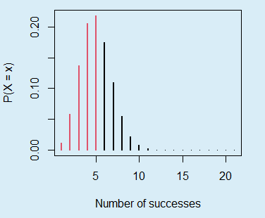
The sum of the probabilities displayed in red is equal to pbinom(5, size = 20, prob = 0.2).
pbinom example
In this section we will review a more complete example to understand how to calculate binomial probabilities in several scenarios. Consider that a basketball player scores 4 out of 10 baskets (\(p = 0.4\)). If the player thows 20 baskets (20 trials):
- The probability of scoring 6 or less baskets, \(P(X \leq 6)\), is:
pbinom(6, size = 20, prob = 0.4) # 0.2500107 or 25%
1 - pbinom(6, size = 20, prob = 0.4, lower.tail = FALSE) # Equivalent
This probability can also be calculated adding the corresponding elements of the binomial probability function, as we pointed out in the previous section:
sum(dbinom(0:6, size = 20, prob = 0.4)) # 0.2500107 or 25%Using the function that we defined before we can represent the calculated probability:
binom_sum(size = 20, prob = 0.4, ub = 6, lwd = 2,
          ylab = "P(X = x)", xlab = "Number of successes")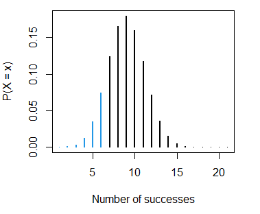
- The probability of scoring less than 6 baskets, \(P(X < 6)\), is:
pbinom(5, size = 20, prob = 0.4) # 0.125599 or 12.56%
1 - pbinom(5, size = 20, prob = 0.4, lower.tail = FALSE) # Equivalent
sum(dbinom(0:5, size = 20, prob = 0.4)) # Equivalent
Note that we set 5 on the first argument of the function instead of 6 because the binomial distribution is discrete, so \(P(X < 6) = P(X \leq 5)\). The calculated probability can be represented with the sum of the following probabilities of the probability mass function:
binom_sum(size = 20, prob = 0.4, ub = 5, lwd = 2,
          ylab = "P(X = x)", xlab = "Number of successes")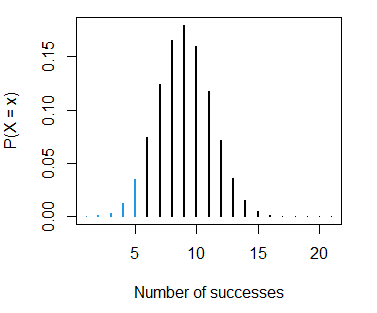
- The probability of scoring more than 12 baskets, \(P(X > 12)\), is:
pbinom(12, size = 20, prob = 0.4, lower.tail = FALSE) # 0.02102893 or 2.1%
1 - pbinom(12, size = 20, prob = 0.4)     # Equivalent
sum(dbinom(13:20, size = 20, prob = 0.4)) # Equivalent
This probability corresponds to:
binom_sum(size = 20, prob = 0.4, lb = 12, lwd = 2,
          ylab = "P(X = x)", xlab = "Number of successes")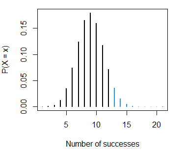
- The probability of scoring between 7 and 11 baskets, \(P(7 \leq X \leq 11)\), is:
pbinom(11, size = 20, prob = 0.4) - pbinom(7, size = 20, prob = 0.4) # 0.5275807 or 52.8%
sum(dbinom(8:11, size = 20, prob = 0.4)) # Equivalent
The corresponding plot can be created with the following code:
binom_sum(size = 20, prob = 0.4, lb = 7, ub = 11, lwd = 2,
          ylab = "P(X = x)", xlab = "Number of successes")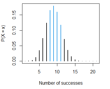
As the binomial distribution is a discrete distribution \(P(X = x) \neq 0\), so \(P(X \geq x) \neq P(X > x)\) and \(P(X \leq x) \neq P(X < x)\).
Plot of the binomial cumulative distribution in R
The binomial distribution function can be plotted in R with the plot function, setting type = “s” and passing the output of the pbinom function for a specific number of experiments and a probability of success.
The following block of code can be used to plot the binomial cumulative distribution functions for 80 trials and different probabilities.
# Grid of X-axis values
x <- 1:80

# size = 80, prob = 0.2
plot(pbinom(x, size = 80, prob = 0.2), type = "s", lwd = 2,
     main = "Binomial distribution function",
     xlab = "Number of successes", ylab = "F(x)")

# size = 80, prob = 0.3
lines(pbinom(x, size = 80, prob = 0.3), type = "s",
      lwd = 2, col = 2)

# size = 80, prob = 0.4
lines(pbinom(x, size = 80, prob = 0.4), type = "s",
      lwd = 2, col = 3)

# Add a legend
legend("bottomright", legend = c("80  0.2", "80  0.3", "80  0.4"),
       title = "size  prob", title.adj = 0.95,
       lty = 1, col = 1:3, lwd = 2, box.lty = 0)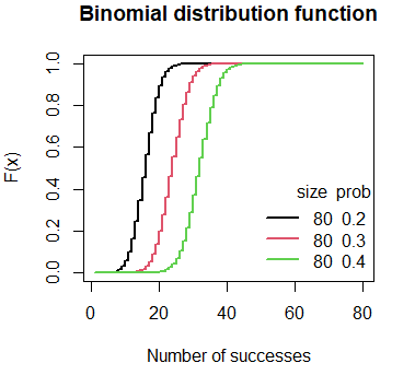
The qbinom function
Given a probability or a set of probabilities, the qbinom function allows you to obtain the corresponding binomial quantile. The following block of code describes briefly the arguments of the function:
qbinom(p,                 # Probability or vector of probabilities
       size,              # Number of trials (n > = 0)
       prob,              # The probability of success on each trial
       lower.tail = TRUE, # If TRUE, probabilities are P(X <= x), or P(X > x) otherwise
       log.p = FALSE)     # If TRUE, probabilities are given as log
As an example, the binomial quantile for the probability 0.4 if \(n = 5\) and \(p = 0.7\) is:
qbinom(p = 0.4, size = 5, prob = 0.7) # 3Plot of the binomial quantile function in R
The binomial quantile function can be plotted in R for a set of probabilities, a number of trials and a probability of success with the following code:
# Grid of X-axis values
x <- 1:80

# size = 80, prob = 0.2
plot(qbinom(seq(0, 1, 0.001), size = 80, prob = 0.2),
     main = "Binomial quantile function",
     ylab = "Q(p)", xlab = "p",
     type = "s", col = 3, xaxt = "n")
axis(1, labels = seq(0, 1, 0.1), at = 0:10 * 100)

# size = 80, prob = 0.3
lines(qbinom(seq(0, 1, 0.001), size = 80, prob = 0.3), type = "s", col = 2)

# size = 80, prob = 0.4
lines(qbinom(seq(0, 1, 0.001), size = 80, prob = 0.4), type = "s", col = 1)

# Add a legend
legend("topleft", legend = c("80  0.2", "80  0.3", "80  0.4"),
       title = "size  prob", title.adj = 0.95,
       lty = 1, col = 1:3, lwd = 2, box.lty = 0)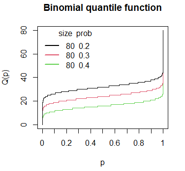
The rbinom function
The rbinom function allows you to draw \(n\) random observations from a binomial distribution in R. The arguments of the function are described below:
rbinom(n,    # Number of random observations to be generated
       size, # Number of trials (> = 0)
       prob) # The probability of success on each trial
If you want to obtain, for instance, 15 random observations from a binomial distribution if the number of trials is 30 and the probability of success on each trial is 0.1 you can type:
rbinom(n = 15, size = 30, prob = 0.1)7 3 2 1 5 1 1 4 4 3 1 5 2 4 1Nonetheless, if you don’t specify a seed before executing the function you will obtain a different set of random observations. If you want to make the output reproducible you can set a seed as follows:
set.seed(2)
rbinom(n = 15, size = 30, prob = 0.1)
2 4 3 1 6 6 1 5 3 3 3 2 4 1 2