For loop in R

The for loop in R, also known as for cycle, is a repetitive iteration in loop of any code, where at each iteration some code is evaluated through the elements of a list or vector.

For loop R syntax

The syntax of the for loop in R is very simple:

for (i in list) {
  # Code
}

It is worth to mention that you could also call a for loop in a single line without brackets. However, this is not the recommended way.

for (i in list) # Code

As a first example, you could think of printing i + 1, being i = 1, ... 5, on each iteration of the loop. In this case, the for loop will start at i = 1 and end at i = 5, so the output will be the following:

for (i in 1:5) {
  print(i + 1)
}

# Equivalent
# for (i in 1:5) print (i + 1) 

2
3
4
5
6

It is important to note that R loops operate over collections rather than iterators. This allows creating loops like the following:

colors <- c("green", "blue", "red")
for (color in colors){
   print(paste0("Color: ", color))
}

"Color: green"
"Color: blue"
"Color: red"

Nested for loop in R

You can also write for loops inside others. This loops are known as nested for cycles. The syntax is represented in the following block code.

for (i in list) {
        # Code
    for(j in list) {
        # Code
    }
}

Examples of R for loops

Bootstrap with the for loop in R

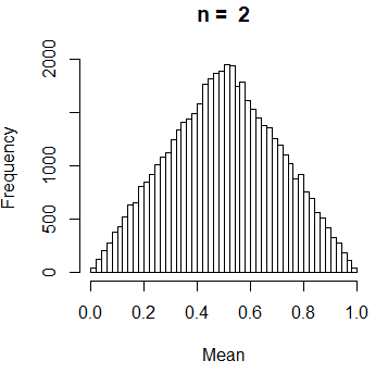
Suppose you want to know the sample mean of n data points obtained independently of a uniform distribution over the interval (0, 1). You can solve the previous problem theoretically, but we are going to do carry out a simulation study. For that purpose we need to follow this simple steps:

1. Generate n data points with uniform distribution in (0, 1).
2. Calculate the sample mean of the data.
3. Repeat the previous steps a high number of repetitions.
4. Approximate the distribution of the sample mean with the histogram obtained with me sample means obtained in the repetitions.

If you are familiar with statistical methods, you may have noticed we are running an uniform bootstrap.

set.seed(1)  # Setting a seed for reproducibility
rep <- 50000 # Number of repetitions
n <- 2       # Number of points

Mean <- numeric(rep)

for (irep in 1:rep) {
    x <- runif(n)
    Mean[irep] <- mean(x)
}


hist(Mean, breaks = 40, main = paste("n = ", n))

Creating a clock with a for cycle

Now, we are going to represent a minute in clock seconds. We recommend you to run this animation in R GUI instead of RStudio, since the refresh rate of the graphics in RStudio is lower.

angle <- seq(0, 360, length = 60)
radians <- angle * pi / 180

x <- cos(radians)
y <- sin(radians)

for (i in 1:60) {
    plot(y, x, axes = F, xlab = "", ylab = "", type = "l", col = "grey")
    arrows(0, 0, y[i], x[i], col = "blue")
    Sys.sleep(1) # Waits one second
}

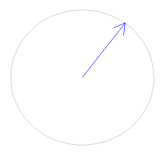
At each iteration, the previous loop plots a clock and after one second it plots the following second and so on. The representation of an iteration is shown in the following image:

Loop break and next functions

Sometimes you need to stop the loop at some index if some condition is met or to avoid evaluating some code for some index or condition. For that, you can use the break and next functions.

In the following example, the loop will break on the sixth iteration (that won’t be evaluated) despite the full loop has 15 iterations, and will also skip the third iteration.

for (iter in 1:15) {

  if (iter == 3) {
        next  
    }

    if (iter == 6) {
        break   
    }

  print(iter)
}

1
2
4
5

Pre-allocate space to run R for loops

Loops are specially slow in R. If you run or plan to run computationally expensive tasks, you must pre-allocate memory. This technique consists on reserving space for the objects you are creating or filling inside a loop. Let’s see an example:

First, you can create a variable named store without indicating the size of the final variable once filled inside the loop. The Sys.time function will store the time when the function itself is executed, so make sure you call the following code at once, not line by line.

start_time <- Sys.time()

store <- numeric()
for (i in 1:1000000){
 store[i] <- i ** 2
}

end_time <- Sys.time()
end_time - start_time  # Time difference of 0.4400518 secs (running time on my computer)

Second, copy the previous code and pre-allocate the store variable with the final length of the vector.

start_time <- Sys.time()

store <- numeric(1000000)

for (i in 1:1000000){
 store[i] <- i ** 2
}

end_time <- Sys.time()
end_time - start_time   # Time difference of 0.126972 secs

Almost 3.5 times faster!

Note that the results may depend on the speed of your computer and will vary if you run the code several times. However, the more resource consuming the task is, the more difference will arise pre-allocating objects in memory. If you try to run the previous codes for only 1000 or 10000 iterations you won’t see the difference.

Vectorized for loop

The foreach function is an alternative of the classical for loop from the foreach package. However, this function is similar to an apply. Note that you will also need to use the %do% operator. This function can make your loops faster, but it could depend on your loop.

In the following example we created a function named for_each where we executed the square root of the corresponding value of each iteration. As the foreach returns a list by default, you can use the .combine argument and set it to 'c' so the output will be concatenated. Other option is to return the result wrapped by the unlist function.

# install.packages("foreach")
library(foreach)

for_each <- function(x) {

    res <- foreach(i = 1:x, .combine = 'c') %do% {
        sqrt(i)
    }

    return(res)
}

for_each(10)

1.000000 1.414214 1.732051 2.000000 2.236068 2.449490 2.645751 2.828427 3.000000 3.162278

Parallel for loop

When dealing with very high resource intensive tasks, like simulation studies, you would need to make your loops parallel. For that, you may need to make use of the parallel and doParallel packages. However, the second package is loaded when you load the first, so you don’t need to call both.

In the following example we set up our parallel execution with all available cores, but you could use as many as you want. Then, register the parallelization and at the end remember to stop your cluster.

library(parallel)

par_for_each <- function(x) {

    cl <- parallel::makeCluster(detectCores())
    doParallel::registerDoParallel(cl) 

    res <- foreach(i = 1:x, .combine = 'c') %dopar% {
        sqrt(i)
    }

  parallel::stopCluster(cl)
  return(res)
}

par_for_each(10)

1.000000 1.414214 1.732051 2.000000 2.236068 2.449490 2.645751 2.828427 3.000000 3.162278