HOME

Contingency table in R

Statistics with R Association of categorical variables

How to create a contingency table in R? The table() function
1. Absolute frequency table in R
2. Relative frequency table in R
Two-way contingency graphs in R
Association measures in R

In several situations it is interesting to study two or more variables at the same time. When working with categorical variables, you can summarize the data in a table called contingency table. The relationship between the variables can be also checked with association measures. In this article you will learn how to create a contingency table in R, how to plot it and verify the grade of relationship between the factor variables with association measures.

How to create a contingency table in R? The table() function

Qualitative variables, also known as nominal, categorical or factor variables appear when you have non-measurable variables (gender, birthplace, race, …). This kind of variables can be represented with text, where each name represents a unique category, or with numbers, where each number represents a unique category. When working with several categorical variables, you can represent its joint frequency distribution with a frequency or contingency table.

Consider the bidimensional case with factor variables $X$ and $Y$ and denote by $x_i$ , $i = 1, \dots, k$ as the different values that can take the variable $X$ and $y_i$ , $i = 1, \dots, h$ as the values that can take the variable $Y$ . With this in mind we can define:

Joint absolute frequency of $(x_i, y_j)$ . Is the number of individuals that represent at the same time the values $x_i \in X$ and $y_j \in Y$ and it is denoted by $n_{ij}$ .
Joint relative frequency. Is the proportion of individuals that represent at the same time the values $x_i \in X$ and $y_j \in Y$ of the total number of individuals and it is defined by $f_{ij} = n{ij}/n$ , where $n$ is the sample size.

Note that the bidimensional distribution is the set of values that the bidimensional variable $(X, Y)$ can take in addition of the joint frequencies of that values. In order to represent a bidimensional distribution you can use a two-way contingency table of the form:

$X$ \ $Y$	$y_1$	$y_2$	$\dots$	$y_j$	$\dots$	$h_h$	$n_{j \bullet}$
$x_1$	$n_{11}$	$n_{12}$	$\dots$	$n_{1j}$	$\dots$	$n_{1h}$	$n_{1 \bullet}$
$x_2$	$n_{21}$	$n_{22}$	$\dots$	$n_{2j}$	$\dots$	$n_{2h}$	$n_{2 \bullet}$
$\vdots$	$\vdots$	$\vdots$	$\ddots$	$\dots$	$\ddots$	$\vdots$	$\vdots$
$x_i$	$n_{i1}$	$n_{i2}$	$\dots$	$n_{ij}$	$\dots$	$n_{ih}$	$n_{i \bullet}$
$\vdots$	$\vdots$	$\vdots$	$\ddots$	$\dots$	$\ddots$	$\vdots$	$\vdots$
$x_k$	$n_{k1}$	$n_{k2}$	$\dots$	$n_{kj}$	$\dots$	$n_{kh}$	$n_{k \bullet}$
$n_{\bullet j}$	$n_{\bullet 1}$	$n_{\bullet 2}$	$\dots$	$n_{\bullet j}$	$\dots$	$n_{\bullet h}$	$n$

Absolute frequency table in R

You can make use of the table function to create a contingency table in R. Consider, for instance, the following example with random data, where the variable $X$ represents the votes for (Yes) and against (No) a law in an international committee composed by members of three different continents (variable $Y$ ):

set.seed(20)

X <- sample(c("Yes", "No"), 10, replace = TRUE)
# "No" "Yes" "Yes" "No"  "No" "Yes" "No" "Yes" "No" "No"

Y <- sample(c("Europe", "America", "Africa"), 10, replace = TRUE)
# "Europe" "Africa"  "Africa"  "Europe"  "Africa" 
# "Europe" "Europe"  "Europe"  "America" "America"

With the table function you can create a frequency table (the marginal distribution) for each variable:

table(X)
# X
#  No Yes 
#   6   4

table(Y)
# Y
#  Africa America  Europe 
#       3       2       5

However, if you pass two variables to the function, you can create a two-way contingency table. It is worth to mention that you could add more variables to the function, resulting into a multidimensional array.

my_table <- table(X, Y)
my_table

Output
     Y
X      Africa  America  Europe
  No       1       2      3
  Yes      2       0      2

Note that you can modify the row and column names of the table with the colnames and rownames functions.

rownames(my_table) <- c("0", "1")
colnames(my_table) <- c("Af", "Am", "Eu")
my_table

Output
   Y
X   Af Am Eu
  0  1  2  3
  1  2  0  2

You can also convert a data frame or a matrix to a table. For that purpose, you could use the as.table function.

Relative frequency table in R

The table created with the table function displays the joint absolute frequency of the variables. Nonetheless, you can create a joint relative frequency table in R (as a fraction of a marginal table) with the prop.table function. By default, the function calculates the proportion of each cell respect to the total of observations, so the sum of the cells is equal to 1.

prop_table <- prop.table(my_table)

Output
     Y
X     Africa  America  Europe
  No     0.1     0.2    0.3
  Yes    0.2     0.0    0.2

However, the margin argument allows you to set the index (1: rows, 2: columns) according to which the proportions are going to be calculated.

On the one hand, if you set margin = 1, the sum of each row will be equal to 1.

prop.table(my_table, margin = 1)

Output
     Y
X        Africa   America    Europe
  No  0.1666667 0.3333333 0.5000000
  Yes 0.5000000 0.0000000 0.5000000

On the other hand, if you specify margin = 2 the relative frequency will be calculated by columns, so each column will sum up to 1.

my_table_2 <- prop.table(my_table, margin = 2)
my_table_2

Output
     Y
X        Africa   America    Europe
  No  0.3333333 1.0000000 0.6000000
  Yes 0.6666667 0.0000000 0.4000000

Note you can also add the margins for a contingency table in R with the addmargins function, to display the cumulative relative frequency (or the cumulative absolute frequency, if you apply it to an absolute frequency table). In the following example we calculate the margins of prop_table, expressing the data as percentage.

my_table_3 <- addmargins(prop_table * 100)
my_table_3

Output
     Y
X      Africa  America  Europe Sum
  0       10      20      30    60
  1       20       0      20    40
  Sum     30      20      50   100

Two-way contingency graphs in R

In order to plot a contingency table in R you can make use of the bar charts with the barplot function. There are two main types: grouped and stacked. By default, the function will create a stacked bar plot:

# Divide the graphical window in two colums
par(mfrow = c(1, 2))

colors <- c("#80FFFF", "#FFFFFF")

barplot(my_table, col = colors)

# Adding a legend
legend("topleft", legend = c("No", "Yes"), fill = colors)

barplot(my_table_2, col = colors)

# Back to the original graphical window
par(mfrow = c(1, 1))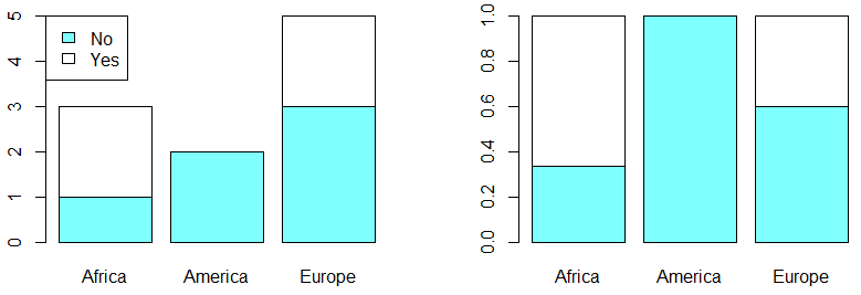

Two way contingency graph in R

If you prefer a grouped bar plot you will need to set the argument beside as TRUE:

par(mfrow = c(1, 2))

barplot(my_table, col = colors, beside = TRUE)
legend("topleft", legend = c("No", "Yes"), fill = colors)
barplot(my_table_2, col = colors, beside = TRUE)

par(mfrow = c(1, 1))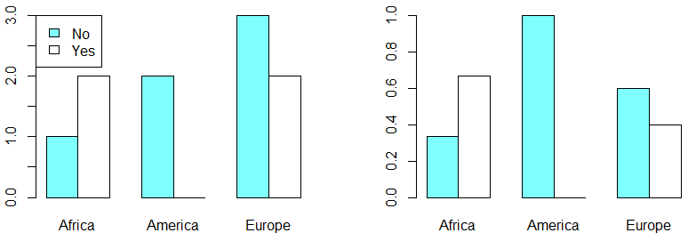

Plot a table in R

An alternative to bar plots are mosaic plots, that allows you to display two or more categorical variables. This kind of plot can be created in base R with the mosaicplot function as follows:

par(mfrow = c(1, 2))

mosaicplot(my_table, cex = 1.1)
mosaicplot(my_table_2, cex = 1.1)

par(mfrow = c(1, 1))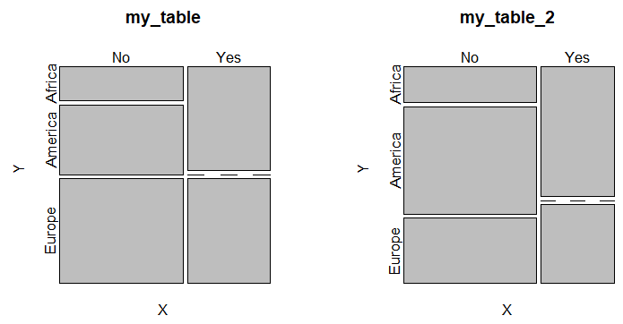

Mosaic plot from table in R

All the boxes across categories having the same area is a signal of independence.

Association measures in R

You can check if the variables are dependent, if there exist some relation between them, or independent if not. In order to define the condition of independence, if $X$ is independent of $Y$ we can check that for all $i$ :

$\frac{n_{i1}}{n_{\bullet 1}} = \frac{n_{i2}}{n_{\bullet 2}} = \dots = \frac{n_{ij}}{n_{\bullet j}} = \dots = \frac{n_{ih}}{n_{\bullet h}} = \frac{n_{i \bullet}}{n}.$

The previous is equivalent to:

$\frac{n_{i j}}{n} = \frac{n_{i \bullet}}{n} \frac{n_{\bullet j}}{n} \quad \forall i, j.$

Chi-square coefficient in R

You can check for independence with the chi-square test, comparing the expected frequencies $e_{ij}$ with $n_{ij}$ . The chi-square metric is:

$\chi^2 = \sum_{i, j} \frac{(n_{ij} - e_{ij})^2}{e_{ij}}.$

Note that this variable provides, in relative terms, the distance between the joint distribution of the variables of the case of independence. Hence, the bigger the value of $\chi^2$ , the greater the association between the variables. This measure goes from 0 (independence case) to $n(q-1)$ , being $q$ the minimum between the number of rows and columns.

However, as this metric is not bounded between 0 and 1 there exists other association measures, described in the following subsections.

You can calculate the Chi-square coefficient in R performing a Chi-square test with the chisq.test function as follows:

chi <- chisq.test(my_table)
chi$statistic

Output
X-squared 
 2.222222

Therefore, in this case, the Chi-square coefficient is 2.2222.

Contingency coefficient

The contingency coefficient C is bounded between 0 (independence) and 1. It is defined as:

$C = \sqrt{\frac{\chi^2}{\chi^2 + n}}.$

In order to calculate the contingency coefficient in R you can make use of the following function:

Contingency <- function(x) {
    chi <- chisq.test(x)
    unname(sqrt(chi$statistic / (chi$statistic + sum(x))))
}

Contingency(my_table) # 0.4264014

An alternative is to use the ContCoef function of the DescTools package:

# install.packages("DescTools")
library(DescTools)

ContCoef(my_table) # 0.4264014

The maximum value that the contingency coefficient can take is $\sqrt{(k-1)/k}$ , so the value 1 is never reached for square tables. Let $k$ be the number of rows and $h$ the number of columns, some values that the coefficient can take are:

k = h	2	3	4	5	6
max C	0.71	0.82	0.87	0.89	0.91

Phi and Cramer’s V coefficients

The Phi coefficient is defined as:

$\phi = \sqrt{\frac{\chi^2}{n}}.$

Note that it takes values between 0 and 1 in tables 2×2. However, it can take values greater than 1 in other cases. In order to avoid that issue, the Cramer’s V coefficient modifies the Phi coefficient, taking the form:

$V = \sqrt{\frac{\chi^2}{[n(q - 1)]}}.$

Recall that $q$ is the minimum between the number of rows and columns.

In R you can make use of the following functions to calculate these coefficients:

# Phi coefficient
PhiCoef <- function(x){
    unname(sqrt(chisq.test(x)$statistic / sum(x)))
}

# Cramer's V coefficient
V <- function(x) {
    unname(sqrt(chisq.test(x)$statistic / (sum(x) * (min(dim(x)) - 1))))
}

PhiCoef(my_table) # 0.4714045
V(my_table)   # 0.4714045

An alternative is to use the Phi and CramerV functions of the DescTools package.

# install.packages("DescTools")
library(DescTools)

Phi(my_table) # 0.4714045
CramerV(my_table) # 0.4714045

As a final remark, it is worth to mention that you can calculate several association measures in R at the same time with the assocstats function of the vcd library.

# install.packages("vcd")
library(vcd)

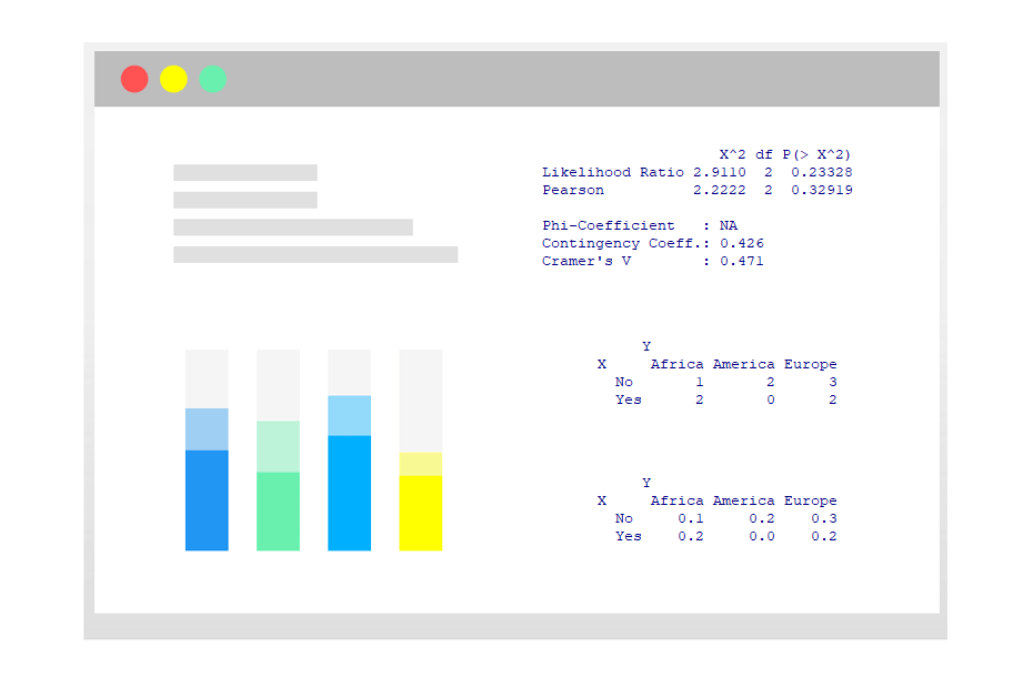
assocstats(my_table)

Output
                    X^2 df P(> X^2)
Likelihood Ratio 2.9110  2  0.23328
Pearson          2.2222  2  0.32919

Phi-Coefficient   : NA 
Contingency Coeff.: 0.426 
Cramer's V        : 0.471