Stem and leaf plot in R
A stem and leaf plot, also known as stem and leaf diagram or stem and leaf display is a classical representation of the distribution of quantitative data, similar to a histogram but in text, where the data is divided into the stem (usually the first or firsts digits of the number) and the leaf (the last digit). The stem and leaf plot in R can be useful when dealing with few observations (15 – 150 data points). In this tutorial you will learn what is a stem and leaf plot and how to make it in R.
How to interpret a stem and leaf plot?
Suppose that you have the following vector:
\(\textbf{x} = (12, 15, 16, 21, 24, 29, 30, 31, 32, 33, \\ \phantom{\textbf{x} = (} 45, 46, 49, 50, 52, 58, 60, 63, 64, 65)\).
In order to manually create a stem plot you have to divide the data into stems (in this case, the first digit of the number) and leafs (the second digit). Hence, the plot will be as follows:
| Stem | Leaf | |
|---|---|---|
| 1 | | | 256 |
| 2 | | | 149 |
| 3 | | | 0123 |
| 4 | | | 569 |
| 5 | | | 058 |
| 6 | | | 0345 |
In consequence, in this example you can read \(1|256\) as 12, 15 and 16, \(2|149\) as 21, 24 and 29 and so on.
The stem is not always a single digit or the first digit of the number. As an example, if you are working with a number with 4 decimal digits, the stem could be the first three decimal digits and the corresponding leaf the fourth, as long as you indicate how digits far is the decimal point from the right of the separator.
The stem function in R
The stem function allows you to create a stem and leaf plot in R. The syntax of the function is as follows:
stem(x,            # Numeric vector
     scale = 1,    # Length of the plot
     width = 80,   # Width of the plot
     atom = 1e-08) # Tolerance parameter
It should be noted that if the input argument contains non-finite or missing values they are not taken into account. Consider, for instance, the following vector:
data <- c(12, 15, 16, 21, 24, 29, 30, 31, 32, 33,
          45, 46, 49, 50, 52, 58, 60, 63, 64, 65)
You can create a simple stem plot typing:
stem(data)The output is the text displayed in the following block. Note that, to clarify, in the comments we show the corresponding values to each stem.
 The decimal point is 1 digit(s) to the right of the |

  0 | 256                 # <-- 12, 15, 16
  2 | 1490123             # <-- 21, 24, 29, 30, 31, 32, 33
  4 | 569028              # <-- 45, 46, 49, 50, 52, 58
  6 | 0345                # <-- 60, 63, 64, 65
However, you may have noticed that the output is not equal to the example we reviewed in the first section. This is due to the stems are grouped (the first stem is for 0 and 1, the second for 2 and 3, and so on). In order to solve this issue you can change the height of the plot with the scale argument as follows:
stem(data, scale = 2)The decimal point is 1 digit(s) to the right of the |
1 | 256 # <-- 12, 15, 16
2 | 149 # <-- 21, 24, 29
3 | 0123 # <-- 30, 31, 32, 33
4 | 569 # <-- 45, 46, 49
5 | 028 # <-- 50, 52, 58
6 | 0345 # <-- 60, 63, 64, 65Note that if you set scale = 3, each stem will be duplicated. In this example, the first of the duplicated stem shows the leafs corresponding to values lower than 5 and the second the leafs corresponding to values equal or higher to 5.
stem(data, scale = 3) The decimal point is 1 digit(s) to the right of the |
1 | 2 # <-- 12
1 | 56 # <-- 15, 16
2 | 14
2 | 9
3 | 0123
3 |
4 |
4 | 569
5 | 02
5 | 8
6 | 034
6 | 5The stem.leaf function
The stem.leaf function of the aplpack library is an alternative to the base R stem function, that allows additional configuration. There are several arguments that can be customized, so refer to the documentation of the function with help(stem.leaf) or ?stem.leaf for additional details. In order to create the stem and leaf diagram with default arguments you can type:
# install.packages("aplpack")
library(aplpack)

stem.leaf(data)
1 | 2: represents 12
leaf unit: 1
n: 20
1 1* | 2
3 1. | 56
5 2* | 14
6 2. | 9
(4) 3* | 0123
3. |
4* |
(3) 4. | 569
7 5* | 02
5 5. | 8
4 6* | 034
1 6. | 5You may have noticed that the output is similar to stem(data, scale = 3). In this case, if you want to customize the number of parts which the stems are divided, you can use the argument m.
stem.leaf(data, m = 1)1 | 2: represents 12
leaf unit: 1
n: 20
3 1 | 256
6 2 | 149
(4) 3 | 0123
(3) 4 | 569
7 5 | 028
4 6 | 0345Comparative (back to back) stem and leaf diagram in R
Other interesting function of the aplpack package is that allows you to compare two stem and leaf plots with the stem.leaf.backback function, that by default plots a back-to-back (two sided) stem and leaf display:
# install.packages("aplpack")
library(aplpack)

set.seed(1)
data2 <- sample(data, replace = TRUE)

stem.leaf.backback(data, data2)
________________________________
1 | 2: represents 12, leaf unit: 1
data data2
________________________________
1 2| 1* |22 2
3 65| 1. |5 3
5 41| 2* |1444 7
6 9| 2. |
(4) 3210| 3* |002233 (6)
| 3. |
| 4* |
(3) 965| 4. |5 7
7 20| 5* |0002 6
5 8| 5. |
4 430| 6* |34 2
1 5| 6. |
| 7* |
________________________________
n: 20 20
________________________________In addition, if you set the argument back.to.back as FALSE, the plots won’t be displayed back-to-back:
stem.leaf.backback(data, data2, back.to.back = FALSE)________________________________
1 | 2: represents 12, leaf unit: 1
data data2
________________________________
1* |2 1 |22 2
1. |56 3 |5 3
2* |14 5 |1444 7
2. |9 6 |
3* |0123 (4) |002233 (6)
3. | |
4* | |
4. |569 (3) |5 7
5* |02 7 |0002 6
5. |8 5 |
6* |034 4 |34 2
6. |5 1 |
7* | |
________________________________
n: 20 20
________________________________Saving a stem and leaf plot as an image
Stem plots are text plots, so they are printed to the console. However, in some situations it is interesting to save the plot as any other plot. Instead of creating a low quality screenshot you can make us of the capture.output function to save the output as character and the paste it to an empty plot with the text function:
# Height and width will depend on your data
windows(width = 4, height = 5)

plot.new()

out <- capture.output(stem(data, scale = 2))
text(0, 1, paste(out, collapse = "n"), adj = c(0, 1))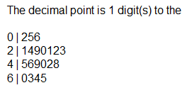
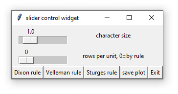
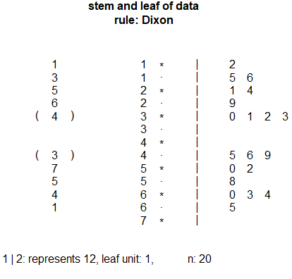
An alternative is to use the function slider.stem.leaf, provided by the tcltk and aplpack packages. This function will open a window to customize in real time the resulting stem and leaf diagram and save it:
# install.packages("tcltk")
library(tcltk)

# install.packages("aplpack")
library(aplpack)

slider.stem.leaf(data)