Create functions in R

R programming language allows the user create their own new functions. In this tutorial you will learn how to write a function in R, how the syntax is, the arguments, the output, how the return function works, and how make a correct use of optional, additional and default arguments.
How to write a function in R language? Defining R functions
The base R functions doesn’t always cover all our needs. In order to write a function in R you first need to know how the syntax of the function command is. The basic R function syntax is as follows:
function_name <- function(arg1, arg2, ... ) {
        # Code
}
In the previous code block we have the following parts:
-
arg1, arg2, …are the input arguments. -
# Coderepresents the code to be executed within the function to calculate the desired output.
The output of the function can be a number, a list, a data.frame, a plot, a message or any object you want. You can also assign the output some class, but we will talk about this in other post with the S3 classes. The last is specially interesting when writing functions for R packages.
Creating a function in R
To introduce R functions we will create a function to work with geometric progressions. A geometric progression is a succession of numbers \(a_1, a_2, a_3\) such that each of them (except the first) is equal to the last multiplied by a constant r called ratio. You can verify that,
\(a_2 = a_1 \cdot r; \qquad a_3 = a_2 \cdot r = a_1 \cdot r^2; \dots\)
Hence, generalizing this process you can obtain the general term
\(a_n = a_1 \cdot r^{n-1}\).
You can also verify that the sum of the n terms of the progression is
\(S_n = a_1 + \dots + a_n = \frac{a_1(r^n - 1)}{r-1}\).
With this in mind you can create the following function,
an <- function(a1, r, n){
    a1 * r ** (n - 1)
}
that calculates the general term \(a_n\) of a geometric progression giving the parameters \(a_1\), the ratio r and the value n. In the following block we can see some examples with its output as comments.
an(a1 = 1, r = 2, n = 5)  # 16
an(a1 = 4, r = -2, n = 6) # -128
With the previous function you can obtain several values of the progression passing a vector of values to the argument n.
an(a1 = 1, r = 2, n = 1:5)   # a_1, ..., a_5
an(a1 = 1, r = 2, n = 10:15) # a_10,..., a_15
You can also calculate the first n elements of the progression with sn function, defined below.
sn <- function(a1, r, n){
    a1 * (r ** n-1)/(r - 1)
}
sn(a1 = 1, r = 2, n = 5) # 31
# Equivalent
values <- an(a1 = 1, r = 2, n = 1:5)
values
sum(values) # 31Input arguments in R functions
Arguments are input values of functions. As an example, on the function we created before we have three input arguments named a1, r and n. There are several considerations when dealing with this type of arguments:
- If you maintain the input order, you don’t need to call the argument names. As an example, the following calls are equivalent.
an(1, 2, 5) # Returns 16
an(a1 = 1, r = 2, n = 5) # Returns 16- If you name the arguments, you can use any order.
an(r = 2, n = 5, a1 = 1) # Returns 16
an(n = 5, r = 2, a1 = 1) # Returns 16-
You can make use of the
argsfunction to know the input arguments of any function you would like to use.
args(an)- If you call the function name, the console will return the code of the function.
Note that sometimes you won’t be able to see the source code of a function if it is not written in R.
Default arguments for functions in R
Sometimes it is very interesting to have default function arguments, so the default values will be used unless others are included when executing the function. When writing a function, such as the one in our example,
function_name <- function(arg1, arg2, arg3 ) {
        # Code
}
if you want arg2 and arg3 to be a and b by default, you can assign them in the arguments of your R function.
function_name <- function(arg1, arg2 = a, arg3 = b) {
        # Code
}
We will illustrate this with a very simple example. Consider, for instance, a function that plots the cosine.
cosine <- function(w = 1, min = -2 * pi, max = 2 * pi) {
    x <- seq(-2 * pi, 2 * pi, length = 200)
    plot(x, cos(w * x), type = "l")
}
Note that this is not the best way to use a function to make a plot. See S3 classes for that purpose.
If you execute cosine() the plot of cos(x) will be plotted by default in the interval [-2π, 2π]. However, if you want to plot the function cos(2x) in the same interval you need to execute cosine(w = 2). Let’s see some examples:
# One row, three columns
par(mfcol = c(1, 3))

cosine()
cosine(w = 2)
cosine(w = 3, min = -3 * pi)
Additional arguments in R
The argument … (dot-dot-dot) allows you to freely pass arguments that will use a sub-function inside the main function. As an example, in the function,
cosine <- function(w = 1, min = -2 * pi, max = 2 * pi, ...) {
    x <- seq(-2 * pi, 2 * pi, length = 200)
    plot(x, cos(w * x), ...)
}
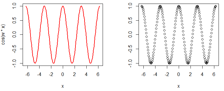
the arguments inside … will be used by the plot function. Let’s see a complete example:
par(mfcol = c(1, 2))

cosine(w = 2, col = "red", type = "l", lwd = 2)
cosine(w = 2, ylab = "")
The R return function
By default, the R functions will return the last evaluated object inside it. You can also make use of the return function, which is especially important when you want to return one object or another, depending on certain conditions, or when you want to execute some code after the object you want to return. It is worth to mention that you can return all types of R objects, but only one. For that reason it is very usual to return a list of objects, as follows:
asn <- function(a1 = 1, r = 2, n = 5) {
    A  <- an(a1, r, n)
    S  <- sn(a1, r, n)
    ii <- 1:n
    AA <- an(a1, r, ii)
    SS <- sn(a1, r, ii)
    return(list(an = A, sn = S,
                output = data.frame(values = AA,
                                    sum = SS)))
}
When you run the function, you will have the following output. Recall to have the sn and an functions loaded in the workspace.
asn()$`an`
[1] 16
$sn
[1] 31
$output
values sum
1 1 1
2 2 3
3 4 7
4 8 15
5 16 31You may have noticed that in the previous case it is equivalent to use the return function or not using it. However, consider the following example, where we want to check whether the parameters passed to the arguments are numbers or not. For this, if any of the parameters is not a number we will return a string, but if they are numbers the code will continue executing.
asn <- function(a1 = 1, r = 2, n = 5) {
    if(!is.numeric(c(a1, r, n))) return("The parameters must be numbers")
    A  <- an(a1, r, n)
    S  <- sn(a1, r, n)
    ii <- 1:n
    AA <- an(a1, r, ii)
    SS <- sn(a1, r, ii)
    return(list(an = A, sn = S,
                output = data.frame(values = AA,
                                    sum = SS)))
}asn("3")"The parameters must be numbers"If we have used the print function instead of return, when some parameter is not numeric, the text will be returned but also an error, since all the code will be executed.
asn <- function(a1 = 1, r = 2, n = 5) {
    if(!is.numeric(c(a1, r, n))) print("The parameters must be numbers")
    A  <- an(a1, r, n)
    S  <- sn(a1, r, n)
    ii <- 1:n
    AA <- an(a1, r, ii)
    SS <- sn(a1, r, ii)
    return(list(an = A, sn = S,
                output = data.frame(values = AA,
                                    sum = SS)))
}asn("3")"The parameters must be numbers"
Error in a1 * r^(n - 1) : non-numeric argument to binary operatorLocal and global variables in R
In R it is not necessary to declare the variables used within a function. The rule called “lexicographic scope” is used to decide whether an object is local to a function or global. Consider, for instance, the following example:
fun <- function() {
    print(x)
}

x<- 1

fun() # 1
The variable x is not defined within fun, so R will search for x within the “surrounding” scope and print its value. If x is used as the name of an object inside the function, the value of x in the global environment (outside the function) does not change.
x <- 1
fun2 <- function() {
    x <- 2
    print(x)
}

fun2() # 2
x #1
To change the global value of a variable inside a function you can use the double assignment operator (<<-).
x <- 1
y <- 3
fun3 <- function() {
    x <- 2
    y <<- 5
    print(paste(x, y))
}

fun3() # 2 5
x # 1 (the value hasn't changed)
y # 5 (the value has changed)
Writing a function in R. Examples
In this section different examples of R functions are shown in order to illustrate the creation and use of R functions.
Example function 1: Letter of Spanish DNI
Let’s calculate the letter of the DNI from its corresponding number. The method used to obtain the letter (L) of the DNI consists of dividing the number by 23 and according to the remainder (R) obtained award the letter corresponding to the following table.
| R | L | R | L | R | L | R | L | |||
|---|---|---|---|---|---|---|---|---|---|---|
| 0 | T | 7 | F | 14 | Z | 21 | K | |||
| 1 | R | 8 | P | 15 | S | 22 | E | |||
| 2 | W | 9 | D | 16 | Q | |||||
| 3 | A | 10 | X | 17 | V | |||||
| 4 | G | 11 | B | 18 | H | |||||
| 5 | M | 12 | N | 19 | L | |||||
| 6 | Y | 13 | J | 20 | C |
The function will be like the following.
DNI <- function(number) {
    letters <- c("T", "R", "W", "A", "G", "M", "Y", "F", "P", "D", "X", "B",
                 "N", "J", "Z", "S", "Q", "V", "H", "L", "C", "K", "E")
    letters <- letters[number %% 23 + 1]
    return(letters)
}
DNI(50247828) # GExample function 2: Throwing a die
The next function simulates n (by default n = 100) dice throws. The function returns the frequency table and the corresponding plot.
dice <- function(n = 100){
    throws <- sample(1:6, n, rep = T)
    frequency <- table(throws)/n
    barplot(frequency, main = "")
    abline(h = 1/6, col = 'red', lwd = 2)
    return(frequency)
}
Now you can see the simulation results executing the function.
par(mfcol = c(1, 3))

dice(100)
dice(500)
dice(100000)
# 100
1 2 3 4 5 6
0.17 0.11 0.20 0.16 0.25 0.11
# 500
1 2 3 4 5 6
0.144 0.158 0.148 0.178 0.164 0.208
# 100000
1 2 3 4 5 6
0.16612 0.16630 0.16569 0.16791 0.16697 0.16701As you can see, as we increase n we are closer to the theoretical value 1/6 = 0.1667.


